<?xml version="1.0" encoding="utf-8"?>
<feed xmlns="http://www.w3.org/2005/Atom">
  <id>https://www.lairdstewart.com/</id>
  <title>Laird Stewart's blog</title>
  <updated>2026-05-22T00:00:00Z</updated>
  <author>
    <name>Laird Stewart</name>
  </author>
  <link rel="self" href="https://www.lairdstewart.com/feed.xml"/>
  <link rel="alternate" href="https://www.lairdstewart.com/"/>
  <icon>resources/icon.png</icon>
  <entry>
    <id>https://www.lairdstewart.com/blog/no-free-lunch-software.html</id>
    <title>There's no free lunch in software</title>
    <updated>2026-05-22T00:00:00Z</updated>
    <link rel="alternate" href="blog/no-free-lunch-software.html"/>
    <content type="xhtml">
      <div xmlns="http://www.w3.org/1999/xhtml">
<p>
      Scott Sumner wrote a good post earlier this month on the
      <a href="https://scottsumner.substack.com/p/the-beauty-of-tautologies"
        >usefulness of tautologies</a
      >
      which got me thinking about tautologies in software development. One which
      came to mind is
    </p>

    <blockquote>
      "To reduce intrinsic complexity of a program one must reduce the
      complexity of the problem it's solving"
    </blockquote>

    <p>
      I liken this to the no free lunch theorem (hence the title of this post)
      because when designing ML algorithms, you can only improve performance by
      limiting the set of problems under consideration (i.e., making assumptions
      about the problem at hand). Similarly, in software, you can only simplify
      code by making simplifying assumptions about the problem you're solving.
    </p>

    <p>
      So what can we learn from this tautology? If you believe that software
      developers should strive for simplicity (as John Ousterhout argues in
      <a
        href="https://www.goodreads.com/en/book/show/39996759-a-philosophy-of-software-design"
        >"A Philosophy of Software Design"</a
      >), then you must also believe software developers should focus on making
      assumptions.
    </p>

    <p>
      What are assumptions to a software engineer? Assertions, preconditions,
      and API contracts! We should therefore strive to write methods that looks
      like
    </p>

    <pre xml:space="preserve"><code>/**
 * Assumes that bar() was called first.
 */
public void foo(Key key)
{
    Preconditions.checkArgument(key != null);
    Preconditions.checkArgument(cache.contains(key));
    Preconditions.checkState(isCacheInitialized());
    ...
}</code></pre>

    <p>
      with the understanding that it will simplify the final program. I've
      recently found myself writing more and more methods that look like this.
      When I started out, I would have looked at comments like
    </p>
    <blockquote>
      "this method assumes that it will only be invoked once"
    </blockquote>
    <p>or</p>
    <blockquote>
      "this only works assuming no more data will be added to this collection"
    </blockquote>
    <p>
      as "cop-outs" or lazy coding, when in reality they are important design
      decisions. Every simplification is the flip-side of an assumption, and
      it's better to document (or code!) assumptions directly than leave them
      implicit.
    </p>
      </div>
    </content>
  </entry>
  <entry>
    <id>https://www.lairdstewart.com/newsletter/april-26.html</id>
    <title>April 2026 Roundup</title>
    <updated>2026-04-01T00:00:00Z</updated>
    <link rel="alternate" href="newsletter/april-26.html"/>
    <content type="xhtml">
      <div xmlns="http://www.w3.org/1999/xhtml">
<!--
        <p>title...</p>
        <div style="padding-left: 1em">
          <blockquote>
            <p lang="en" dir="ltr">
              quote, quote, quote
            </p>
          </blockquote>
          <a href="https://www.google.com">article title</a>, author, 1/1/26
        </div>
        <br />
        -->

        <p>A demand-side analysis of AI's impact on the job market</p>
        <div style="padding-left: 1em">
          <p>
            This is the best article I've read since starting this newsletter.
            If you click on one link, make it this one.
          </p>
          <blockquote>
            <p lang="en" dir="ltr">
              As people get richer, they don’t just want more commodities. They
              want things that aren’t commodities in the standard sense of the
              word. The social aspects of products such as the relationships,
              the status, and exclusivity—what Rene Girard called the mimetic
              properties of desire—become much more relevant once people’s basic
              needs are satisfied. And the demand for these properties will
              bring the human element back into the production process, and with
              it, the jobs.
            </p>
          </blockquote>
          <blockquote>
            <p lang="en" dir="ltr">
              When AI automates commodity production, prices in that sector
              fall. That raises real income. If the goods and services people
              want more of as they get richer lie disproportionately in the
              relational sector, demand shifts in that direction. Baumol’s cost
              disease then amplifies the result: if the relational sector
              remains harder to automate, it becomes relatively more expensive
              and absorbs a growing share of total expenditure.
            </p>
          </blockquote>
          <a href="https://aleximas.substack.com/p/what-will-be-scarce"
            >What will be scarce?</a
          >, Alex Imas, 4/14/26
        </div>
        <br />

        <p>If you collaborate using Git, here are some fun commands to run</p>
        <div style="padding-left: 1em">
          <pre xml:space="preserve"><code>git log --format=format: --name-only --since="1 year ago" | sort | uniq -c | sort -nr | head -20</code>
git shortlog -sn --no-merges
git log --format='%ad' --date=format:'%Y-%m' | sort | uniq -c
          </pre>
          <a href="https://piechowski.io/post/git-commands-before-reading-code/"
            >The Git Commands I Run Before Reading Any Code</a
          >, Ally Piechowski, 4/8/26
        </div>
        <br />

        <p>One Dimensional chess</p>
        <div style="padding-left: 1em">
          <img src="/resources/newsletter/apr-26/1d-chess.png" />
          <a href="https://rowan441.github.io/1dchess/chess.html">1D-Chess</a>,
          Rowan Monk
        </div>
        <br />

        <p>Frontier AI labs are profitable on the margin</p>
        <div style="padding-left: 1em">
          <p>
            I had a discussion this week with co-workers about future AI cost
            for consumers. They argued that the model companies aren't
            profitable, and that they will inevitably raise prices to recoup
            their investments. This is a suspect claim, but apparently popular
            among otherwise well-informed people, so I thought I'd address it
            here. Two important pieces of information
          </p>
          <ol>
            <li>
              Holding capability constant, inference cost has fallen 10x-100x
              year over year
            </li>
            <li>
              While providers are operating at net losses, they are profitable
              on the margin
            </li>
          </ol>

          <p>
            Micro 101 tells us that the firms will serve their models at the
            point where marginal cost equals marginal revenue. Importantly,
            upfront costs don't affect this equilibrium. Even if OpenAI were a
            monopoly and faced no competition, so long as the elasticity of
            demand is not 0, if marginal costs decrease, part of those savings
            will be passed along to consumers.
          </p>
          <p>
            <a href="https://epoch.ai/data-insights/llm-inference-price-trends"
              >LLM inference prices have fallen rapidly but unequally across
              tasks</a
            >, EpochAI, 3/12/25
            <br />
            <a
              href="https://martinalderson.com/blog/no-it-doesnt-cost-anthropic-5k-per-claude-code-user/"
              >No, it doesn't cost Anthropic $5k per Claude Code user</a
            >, Martin Alderson, 3/9/26
          </p>
        </div>
      </div>
    </content>
  </entry>
  <entry>
    <id>https://www.lairdstewart.com/newsletter/march-26.html</id>
    <title>March 2026 Roundup</title>
    <updated>2026-03-01T00:00:00Z</updated>
    <link rel="alternate" href="newsletter/march-26.html"/>
    <content type="xhtml">
      <div xmlns="http://www.w3.org/1999/xhtml">
<p>Grade inflation hurts students in the long run</p>
        <div style="padding-left: 1em">
          <blockquote>
            <p lang="en" dir="ltr">
              Being assigned a higher average grade inflating teacher reduces a
              student's future test scores, the likelihood of graduating from
              high school, college enrollment, and ultimately earnings. ...The
              cumulative impact is economically significant: a teacher with one
              standard deviation higher average grade inflation reduces the
              present discounted value of lifetime earnings of their students by
              $213,872 per year.
            </p>
          </blockquote>
          <a href="https://www.nber.org/papers/w34952"
            >Easy A's, Less Pay: The Long-Term Effects of Grade Inflation</a
          >, NBER, 3/2026
        </div>
        <br />

        <p>
          Related, one proposed solution to grade inflation: capping the number
          of A grades awardable, penalizes students for taking difficult
          courses.
        </p>
        <div style="padding-left: 1em">
          <blockquote>
            <p lang="en" dir="ltr">
              The real problem is not inflation per se. It’s that students are
              penalized for taking harder courses with stronger peers. A grade
              cap leaves that distortion intact—and can even amplify it.
              <br />
              ...
              <br />
              The underlying issue is informational. A grade tries to capture
              two things—student ability and course difficulty—with a single
              number. Gans and Kominers show that in general this is impossible:
              if some students take math and earn B’s while others take
              political science and earn A’s, there is no way, from grades
              alone, to tell whether the difference reflects ability or course
              difficulty.
            </p>
          </blockquote>
          <a
            href="https://marginalrevolution.com/marginalrevolution/2026/03/grade-caps-are-not-a-good-solution-to-grade-inflation.html?utm_source=rss&amp;utm_medium=rss&amp;utm_campaign=grade-caps-are-not-a-good-solution-to-grade-inflation"
            >Grade Caps are Not a Good Solution to Grade Inflation</a
          >, Marginal Revolution, 3/30/2026
        </div>
        <br />

        <p>
          Malus provides "clean room as a service" (i.e., the removal of
          external dependencies from a software project)
        </p>
        <div style="padding-left: 1em">
          <blockquote>
            <p lang="en" dir="ltr">
              Our proprietary AI robots independently recreate any open source
              project from scratch. The result? Legally distinct code with
              corporate-friendly licensing. No attribution. No copyleft. No
              problems.
            </p>
          </blockquote>
          This is a consequence of zero-cost software I hadn't considered. An
          important question is whether the negative effects of this on the open
          source ecosystem will be outweighed by the increase in AI-assisted
          contributions. Also raises some interesting legal questions.
          <br />
          <a href="https://malus.sh">https://malus.sh</a>
        </div>
        <br />

        <!--
        <p>
          Cris Arnade is known for having walked many cities around the world.
          He was one of the better recent guests on Conversations with Tyler.
          Here's his much-shared perspective on American public disorder.
        </p>
        <div style="padding-left: 1em">
          <blockquote>
            <p lang="en" dir="ltr">
              I walked twelve miles through Seoul yesterday, and I saw zero
              destitute people. Certainly no homeless. I did see the same group
              of drunk men I always see, playing cards near the river, because
              Koreans drink an immense amount, but as far as daytime drunks go,
              their behavior was exemplary. When they had to piss, they walked
              the two hundred yards to the bathroom, which they left as clean as
              when they came. When they threw away their empty bottles, they
              collected them and walked it to the trash can, even putting them
              into the correct bin.
            </p>
          </blockquote>
          <a
            href="https://walkingtheworld.substack.com/p/america-and-public-disorder"
            >America and Public Disorder</a
          >, Chris Arnade, 3/9/2026
        </div>
        <br />
        -->

        <p>
          Robin Hanson's "Grabby Aliens" model (2020) suggests that if humans
          stay put on Earth, we won't discover aliens for 500 million years
          (median estimate) but once we do, it will only be a few years before
          they arrive on our doorstep. Fun idea.
        </p>
        <div style="padding-left: 1em">
          <blockquote>
            <p lang="en" dir="ltr">
              I think this factor is under-estimated when discussing the Fermi
              Paradox. If most of the planets in the universe are too far away
              for us to see alien life, then if we see it at all we’ll be seeing
              their space ships as they come to us. But we won’t even see them
              launch to us, even with perfect telescopes staring out into the
              galaxy, until they’re almost here. In practice this means that, in
              the grand scheme of human history, the phase between becoming
              aware of aliens and meeting them is vanishingly short.
            </p>
          </blockquote>
          <a
            href="https://caseyhandmer.wordpress.com/2026/03/03/notes-on-the-fermi-paradox/"
            >Notes on the Fermi Paradox</a
          >, Casey Handmer, 3/3/2026
          <br />
          <a
            href="https://www.overcomingbias.com/p/how-far-aggressive-alienshtml"
            >How Far to Grabby Aliens?</a
          >, Robin Hanson, 12/2020
        </div>
        <br />

        <p>
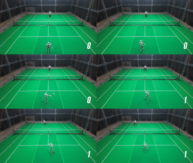
          Trained to play tennis, humanoid robots can hold a cooperative rally.
        </p>
        <div style="padding-left: 1em">
          <img src="/resources/newsletter/march-26/robot-tennis.gif" />
          <br />

          This is the most recent jaw-dropping robotics demo I've seen. The
          footwork is particularly impressive.
          <br />
          <a href="https://zzk273.github.io/LATENT/"
            >LATENT: Learning Athletic Humanoid Tennis Skills from Imperfect
            Human Motion Data</a
          >, 3/13/26
        </div>
        <br />

        <p>
          When it comes to AI's economic impact,
          <a
            href="https://www.econlib.org/archives/2015/02/always_keep_you.html"
            >always keep your eye on production </a
          >.
        </p>
        <div style="padding-left: 1em">
          <blockquote>
            <p lang="en" dir="ltr">
              The real issue is not “Who will get the profits from AI?”; the
              most interesting question is whether AI will lead to the
              production of 130 million household servant robots, or the
              production of another 2000 mega-yachts. When examining issues of
              inequality, it often makes more sense to focus on the structure of
              output, not the distribution of income.
              <br />
              ...
              <br />
              I often see discussions of AI that makes a similar error, failing
              to understand that the essential question is output, not
              distribution. Many worriers about AI don’t seem to understand that
              these two scenarios are almost identical:
              <br />
              <br />
              1. What if AI replaces all jobs?
              <br />
              2. What if America becomes so rich that we can all live as
              billionaires?
            </p>
          </blockquote>
          <a
            href="https://scottsumner.substack.com/p/imagine-130000000-washing-machines"
            >Imagine 130,000,000 Washing Machines</a
          >, Scott Sumner, 01/01/2026
          <br />
        </div>
        <br />

        <p>
          Brain-drain to the U.S. has significantly slowed Canada's economic
          growth
        </p>
        <div style="padding-left: 1em">
          <blockquote>
            <p lang="en" dir="ltr">
              From 2014 to 2024, Canada’s real GDP per capita adjusted for
              purchasing power parity grew by just 3.2 percent in total, an
              anemic 0.4 percent per year on average, and the third lowest among
              38 advanced nations. Over the same period, the United States
              posted 20.2 percent total growth (1.9 percent annually), and the
              OECD average reached 15.3 percent (1.4 percent annually). The
              measurement shortcomings cannot explain five-to six-fold
              differences in growth rates.
              <br />
              ...
              <br />

              The analysis estimates that a substantial share of Canadians who
              would rank among top earners in Canada have emigrated to the
              United States—roughly 40 percent of potential top 1 percent
              earners and 30 to 50 percent of the next nine percentiles.
              Canadian-born individuals in the United States are more educated
              than native-born Americans, earn substantially more, and cluster
              disproportionately in top income deciles.
              <br />
              ...
              <br />

              Canada is effectively exporting its inequality to the U.S. The
              brain drain simultaneously lowers our average income while raising
              American income, accounting for a significant share of the
              persistent GDP gap.
            </p>
          </blockquote>
          <a
            href="https://thehub.ca/2026/03/20/why-canadas-gdp-per-capita-crisis-is-real-deepdive/"
            >Why Canada's GDP per capita crisis is real: DeepDive</a
          >, The Hub, 03/20/2026
          <br />
        </div>
      </div>
    </content>
  </entry>
  <entry>
    <id>https://www.lairdstewart.com/blog/particle-filter.html</id>
    <title>Motivating the Particle Filter</title>
    <updated>2026-02-26T00:00:00Z</updated>
    <link rel="alternate" href="blog/particle-filter.html"/>
    <content type="xhtml">
      <div xmlns="http://www.w3.org/1999/xhtml">
<p>I’ve spent a while searching for resources to provide new
        hires on particle filters. There are two main categories:
        theoretical introductions (e.g., <a
        href="https://www.irisa.fr/aspi/legland/ref/arulampalam02a.pdf">A
        Tutorial on Particle Filters for Online Nonelinear/Non-Gaussian
        Bayesian Tracking</a> and conceptual blog posts (e.g., <a
        href="https://sassafras13.github.io/PF/">Emma Benjaminson’s
        Series</a>). I’ve yet to find a resource with the following
        characteristics</p>
        <ol type="1">
        <li>Accessible to a Math/CS undergrad</li>
        <li>Follows a single example, from Bayesian Inference to a
        Kalman Filter</li>
        <li>Has visualizations of multiple-dimensions and hidden
        variables</li>
        <li>Demonstrates the problems Kalman and Histogram filters
        encounter</li>
        </ol>
        <p>I hope to fill that gap. These notes grew out of a recruiting
        talk I gave at UIUC and are intended as a conceptual primer for
        one of the theoretical introductions. A familiarity with
        calculus, statistics, and linear algebra is useful.</p>
        <h3 id="outline">Outline</h3>
        <p>I’ll follow a single, unifying example: Imagine we’re in a
        submarine equipped with active sonar. Like a bat, we can emit a
        sound and listen for its echo. Given the echo’s elapsed time and
        speed of sound, we can calculate our distance to things.
        Unfortunately, we don’t have a perfect knowledge of the speed of
        sound underwater, as it varies depending on temperature,
        salinity, and depth. We are tasked to find another submarine
        which is somewhere nearby. We’ll start with the simplest case:
        Both submarines are stationary and we want to estimate only the
        distance to the other submarine.</p>
        <p>Each act builds on the previous by adding one layer of
        complexity. A new technique (and limitations of the old one if
        applicable) will be discussed at each stage</p>
        <table>
        <colgroup>
        <col style="width: 3%" />
        <col style="width: 62%" />
        <col style="width: 33%" />
        </colgroup>
        <thead>
        <tr>
        <th style="text-align: left;">Act</th>
        <th style="text-align: left;">Added complexity</th>
        <th style="text-align: left;">Topic</th>
        </tr>
        </thead>
        <tbody>
        <tr>
        <td style="text-align: left;">1</td>
        <td style="text-align: left;">Single measurement, stationary
        submarine (Baseline)</td>
        <td style="text-align: left;">Bayesian Inference</td>
        </tr>
        <tr>
        <td style="text-align: left;">2</td>
        <td style="text-align: left;">Multiple measurements</td>
        <td style="text-align: left;">Recursive Bayesian Inference</td>
        </tr>
        <tr>
        <td style="text-align: left;">3</td>
        <td style="text-align: left;">Moving submarine</td>
        <td style="text-align: left;">Kalman Filter</td>
        </tr>
        <tr>
        <td style="text-align: left;">4</td>
        <td style="text-align: left;">Non-Gaussian prior</td>
        <td style="text-align: left;">Histogram Filter</td>
        </tr>
        <tr>
        <td style="text-align: left;">5</td>
        <td style="text-align: left;">Tracking more dimensions than
        range (e.g., lat, lon)</td>
        <td style="text-align: left;">Particle Filter</td>
        </tr>
        </tbody>
        </table>
        <p>Act 0 provides a recap of Bayes’ rule. Act 6 describes
        resampling and perturbations: two heuristics for better
        performance with less computation.</p>
        <h3 id="act-0-math-recap">Act 0: Math Recap</h3>
        <p>The easiest way to remind yourself of Bayes’ theorem is to
        re-arrange the law of conditional probability (the comma means
        “and”, and the bar means “given”):</p>
        <p><math display="block" xmlns="http://www.w3.org/1998/Math/MathML"><semantics><mrow><mi>P</mi><mo stretchy="false" form="prefix">(</mo><mi>A</mi><mo>,</mo><mi>B</mi><mo stretchy="false" form="postfix">)</mo><mo>=</mo><mi>P</mi><mo stretchy="false" form="prefix">(</mo><mi>A</mi><mo stretchy="false" form="prefix">|</mo><mi>B</mi><mo stretchy="false" form="postfix">)</mo><mi>P</mi><mo stretchy="false" form="prefix">(</mo><mi>B</mi><mo stretchy="false" form="postfix">)</mo><mo>=</mo><mi>P</mi><mo stretchy="false" form="prefix">(</mo><mi>B</mi><mo stretchy="false" form="prefix">|</mo><mi>A</mi><mo stretchy="false" form="postfix">)</mo><mi>P</mi><mo stretchy="false" form="prefix">(</mo><mi>A</mi><mo stretchy="false" form="postfix">)</mo></mrow><annotation encoding="application/x-tex">P(A, B) = P(A|B)P(B) = P(B|A)P(A)</annotation></semantics></math></p>
        <p><math display="block" xmlns="http://www.w3.org/1998/Math/MathML"><semantics><mrow><mi>P</mi><mo stretchy="false" form="prefix">(</mo><mi>A</mi><mo stretchy="false" form="prefix">|</mo><mi>B</mi><mo stretchy="false" form="postfix">)</mo><mo>=</mo><mfrac><mrow><mi>P</mi><mo stretchy="false" form="prefix">(</mo><mi>B</mi><mo stretchy="false" form="prefix">|</mo><mi>A</mi><mo stretchy="false" form="postfix">)</mo><mi>P</mi><mo stretchy="false" form="prefix">(</mo><mi>A</mi><mo stretchy="false" form="postfix">)</mo></mrow><mrow><mi>P</mi><mo stretchy="false" form="prefix">(</mo><mi>B</mi><mo stretchy="false" form="postfix">)</mo></mrow></mfrac></mrow><annotation encoding="application/x-tex">P(A|B)=\frac{P(B|A)P(A)}{P(B)}</annotation></semantics></math></p>
        <p>Bayesian inference is a technique which repeatedly uses
        Bayes’ theorem to understand some outcome/event of interest
        <math display="inline" xmlns="http://www.w3.org/1998/Math/MathML"><semantics><mrow><mo stretchy="false" form="prefix">(</mo><mi>A</mi><mo stretchy="false" form="postfix">)</mo></mrow><annotation encoding="application/x-tex">(A)</annotation></semantics></math> as we observe
        events/collect data which tells us something about it <math display="inline" xmlns="http://www.w3.org/1998/Math/MathML"><semantics><mrow><mo stretchy="false" form="prefix">(</mo><mrow><mtext mathvariant="normal">e.g., </mtext><mspace width="0.333em"></mspace></mrow><mi>B</mi><mo stretchy="false" form="postfix">)</mo></mrow><annotation encoding="application/x-tex">(\textrm{e.g., } B)</annotation></semantics></math>. For example,
        <em>“given that a card is red, what is the probability it is a
        heart?”</em></p>
        <ul>
        <li><math display="inline" xmlns="http://www.w3.org/1998/Math/MathML"><semantics><mrow><mi>P</mi><mo stretchy="false" form="prefix">(</mo><mi>A</mi><mo stretchy="false" form="postfix">)</mo></mrow><annotation encoding="application/x-tex">P(A)</annotation></semantics></math> is called the prior.
        This is the initial degree of belief in the hypothesis <math display="inline" xmlns="http://www.w3.org/1998/Math/MathML"><semantics><mi>A</mi><annotation encoding="application/x-tex">A</annotation></semantics></math>.</li>
        <li><math display="inline" xmlns="http://www.w3.org/1998/Math/MathML"><semantics><mrow><mi>P</mi><mo stretchy="false" form="prefix">(</mo><mi>A</mi><mo stretchy="false" form="prefix">|</mo><mi>B</mi><mo stretchy="false" form="postfix">)</mo></mrow><annotation encoding="application/x-tex">P(A|B)</annotation></semantics></math> is called the
        posterior. It is the degree of belief in <math display="inline" xmlns="http://www.w3.org/1998/Math/MathML"><semantics><mi>A</mi><annotation encoding="application/x-tex">A</annotation></semantics></math> after incorporating the news of
        <math display="inline" xmlns="http://www.w3.org/1998/Math/MathML"><semantics><mi>B</mi><annotation encoding="application/x-tex">B</annotation></semantics></math>.</li>
        <li><math display="inline" xmlns="http://www.w3.org/1998/Math/MathML"><semantics><mrow><mi>P</mi><mo stretchy="false" form="prefix">(</mo><mi>B</mi><mo stretchy="false" form="prefix">|</mo><mi>A</mi><mo stretchy="false" form="postfix">)</mo></mrow><annotation encoding="application/x-tex">P(B|A)</annotation></semantics></math> is the likelihood.
        It is the probability of the data given the hypothesis</li>
        <li><math display="inline" xmlns="http://www.w3.org/1998/Math/MathML"><semantics><mrow><mi>P</mi><mo stretchy="false" form="prefix">(</mo><mi>B</mi><mo stretchy="false" form="postfix">)</mo></mrow><annotation encoding="application/x-tex">P(B)</annotation></semantics></math> is called the
        evidence, or marginal likelihood. It is the probability of the
        data under all hypotheses.</li>
        </ul>
        <p>The crux of Bayesian inference is that once we have <math display="inline" xmlns="http://www.w3.org/1998/Math/MathML"><semantics><mrow><mi>P</mi><mo stretchy="false" form="prefix">(</mo><mi>A</mi><mo stretchy="false" form="prefix">|</mo><mi>B</mi><mo stretchy="false" form="postfix">)</mo></mrow><annotation encoding="application/x-tex">P(A|B)</annotation></semantics></math>, if we observe another event,
        <math display="inline" xmlns="http://www.w3.org/1998/Math/MathML"><semantics><mi>C</mi><annotation encoding="application/x-tex">C</annotation></semantics></math> (which is independent of
        <math display="inline" xmlns="http://www.w3.org/1998/Math/MathML"><semantics><mi>B</mi><annotation encoding="application/x-tex">B</annotation></semantics></math>) we can “update” our belief
        about <math display="inline" xmlns="http://www.w3.org/1998/Math/MathML"><semantics><mi>A</mi><annotation encoding="application/x-tex">A</annotation></semantics></math> by making <math display="inline" xmlns="http://www.w3.org/1998/Math/MathML"><semantics><mrow><mi>P</mi><mo stretchy="false" form="prefix">(</mo><mi>A</mi><mo stretchy="false" form="prefix">|</mo><mi>B</mi><mo stretchy="false" form="postfix">)</mo></mrow><annotation encoding="application/x-tex">P(A|B)</annotation></semantics></math> our prior and starting again
        to find a new posterior, <math display="inline" xmlns="http://www.w3.org/1998/Math/MathML"><semantics><mrow><mi>P</mi><mo stretchy="false" form="prefix">(</mo><mi>A</mi><mo stretchy="false" form="prefix">|</mo><mi>B</mi><mo>,</mo><mi>C</mi><mo stretchy="false" form="postfix">)</mo></mrow><annotation encoding="application/x-tex">P(A|B,C)</annotation></semantics></math>. Note that we don’t have to
        start from scratch each time we get additional evidence, only
        compute Bayes’ theorem one more time. All of our knowledge thus
        far about <math display="inline" xmlns="http://www.w3.org/1998/Math/MathML"><semantics><mi>A</mi><annotation encoding="application/x-tex">A</annotation></semantics></math> is contained in the
        posterior.</p>
        <p>What do I mean by “degree of belief”? If you haven’t come
        across the distinction between Frequentest and Bayesian
        statistics, a frequentest will take a weighted coin, and will
        say “flip it 1 million times, and the ratio of <math display="inline" xmlns="http://www.w3.org/1998/Math/MathML"><semantics><mfrac><mtext mathvariant="normal">#heads</mtext><mtext mathvariant="normal">#flips</mtext></mfrac><annotation encoding="application/x-tex">\frac{\text{\#heads}}{\text{\#flips}}</annotation></semantics></math>
        is the probability it lands heads. A Bayesian will take a
        weighted coin and say probability is the”degree of belief” I
        hold that it will land heads. i.e., if I had to place a bet on
        it, what “probability” would make for a fair betting line?</p>
        <p>We can derive Bayes’ theorem for probability density
        functions similarly:</p>
        <p><math display="block" xmlns="http://www.w3.org/1998/Math/MathML"><semantics><mrow><msub><mi>f</mi><mrow><mi>X</mi><mo>,</mo><mi>Y</mi></mrow></msub><mo stretchy="false" form="prefix">(</mo><mi>x</mi><mo>,</mo><mi>y</mi><mo stretchy="false" form="postfix">)</mo><mo>=</mo><msub><mi>f</mi><mrow><mi>X</mi><mo stretchy="false" form="prefix">|</mo><mi>Y</mi><mo>=</mo><mi>y</mi></mrow></msub><mo stretchy="false" form="prefix">(</mo><mi>x</mi><mo stretchy="false" form="postfix">)</mo><msub><mi>f</mi><mi>Y</mi></msub><mo stretchy="false" form="prefix">(</mo><mi>y</mi><mo stretchy="false" form="postfix">)</mo><mo>=</mo><msub><mi>f</mi><mrow><mi>Y</mi><mo stretchy="false" form="prefix">|</mo><mi>X</mi><mo>=</mo><mi>x</mi></mrow></msub><mo stretchy="false" form="prefix">(</mo><mi>y</mi><mo stretchy="false" form="postfix">)</mo><msub><mi>f</mi><mi>X</mi></msub><mo stretchy="false" form="prefix">(</mo><mi>x</mi><mo stretchy="false" form="postfix">)</mo></mrow><annotation encoding="application/x-tex">f_{X,Y}(x,y)=f_{X|Y=y}(x)f_Y(y)=f_{Y|X=x}(y)f_X(x)</annotation></semantics></math></p>
        <p><math display="block" xmlns="http://www.w3.org/1998/Math/MathML"><semantics><mrow><msub><mi>f</mi><mrow><mi>X</mi><mo stretchy="false" form="prefix">|</mo><mi>Y</mi><mo>=</mo><mi>y</mi></mrow></msub><mo stretchy="false" form="prefix">(</mo><mi>x</mi><mo stretchy="false" form="postfix">)</mo><mo>=</mo><mfrac><mrow><msub><mi>f</mi><mrow><mi>Y</mi><mo stretchy="false" form="prefix">|</mo><mi>X</mi><mo>=</mo><mi>x</mi></mrow></msub><mo stretchy="false" form="prefix">(</mo><mi>y</mi><mo stretchy="false" form="postfix">)</mo><msub><mi>f</mi><mi>X</mi></msub><mo stretchy="false" form="prefix">(</mo><mi>x</mi><mo stretchy="false" form="postfix">)</mo></mrow><mrow><msub><mi>f</mi><mi>Y</mi></msub><mo stretchy="false" form="prefix">(</mo><mi>y</mi><mo stretchy="false" form="postfix">)</mo></mrow></mfrac></mrow><annotation encoding="application/x-tex">f_{X|Y=y}(x)=\frac{f_{Y|X=x}(y)f_X(x)}{f_Y(y)}</annotation></semantics></math></p>
        <p>Remember the evidence, <math display="inline" xmlns="http://www.w3.org/1998/Math/MathML"><semantics><mrow><msub><mi>f</mi><mi>Y</mi></msub><mo stretchy="false" form="prefix">(</mo><mi>y</mi><mo stretchy="false" form="postfix">)</mo></mrow><annotation encoding="application/x-tex">f_Y(y)</annotation></semantics></math>, is the probability density of
        the data under all hypothesis (possible values of <math display="inline" xmlns="http://www.w3.org/1998/Math/MathML"><semantics><mi>x</mi><annotation encoding="application/x-tex">x</annotation></semantics></math>). In the continuous case you would
        write this as an integral</p>
        <p><math display="block" xmlns="http://www.w3.org/1998/Math/MathML"><semantics><mrow><msub><mi>f</mi><mi>Y</mi></msub><mo stretchy="false" form="prefix">(</mo><mi>y</mi><mo stretchy="false" form="postfix">)</mo><mo>=</mo><mo>∫</mo><msub><mi>f</mi><mrow><mi>Y</mi><mo stretchy="false" form="prefix">|</mo><mi>X</mi><mo>=</mo><mi>x</mi></mrow></msub><mo stretchy="false" form="prefix">(</mo><mi>y</mi><mo stretchy="false" form="postfix">)</mo><msub><mi>f</mi><mi>X</mi></msub><mo stretchy="false" form="prefix">(</mo><mi>x</mi><mo stretchy="false" form="postfix">)</mo><mi>d</mi><mi>x</mi></mrow><annotation encoding="application/x-tex">f_Y(y)=\int f_{Y|X=x}(y)f_X(x)dx</annotation></semantics></math></p>
        <h3 id="act-1-one-measurement-of-a-stationary-submarine">Act 1:
        One Measurement of A Stationary Submarine</h3>
        <p>To our submarine example, let’s make the following
        simplifications:</p>
        <ul>
        <li>The problem is one-dimensional</li>
        <li>Both submarines are stationary</li>
        <li>The sonar readings are centered on the true distance with
        some noise. To be precise, they follow the normal distribution
        with <math display="inline" xmlns="http://www.w3.org/1998/Math/MathML"><semantics><mrow><mi>μ</mi><mo>=</mo><mtext mathvariant="normal">true distance</mtext></mrow><annotation encoding="application/x-tex">\mu=\text{true distance}</annotation></semantics></math>,
        and <math display="inline" xmlns="http://www.w3.org/1998/Math/MathML"><semantics><mrow><mi>σ</mi><mo>=</mo><mn>100</mn></mrow><annotation encoding="application/x-tex">\sigma=100</annotation></semantics></math>. A positive
        value means the object is in front, negative means it is
        behind.</li>
        </ul>
        <pre xml:space="preserve"><code>   🛥️ ········))       🛥️
&lt;───┼───────────────────┼───&gt; x
    0                  ❓</code></pre>
        <p>Given the following measurement</p>
        <!-- truth: 4900 meters -->
        <table>
        <thead>
        <tr>
        <th style="text-align: left;">Measurement</th>
        <th style="text-align: center;">Range</th>
        </tr>
        </thead>
        <tbody>
        <tr>
        <td style="text-align: left;">#1</td>
        <td style="text-align: center;">4781 meters</td>
        </tr>
        </tbody>
        </table>
        <p>what is the probability distribution of position of the other
        sub? Let’s approach this as a Bayesian. Call the distance to the
        other submarine <math display="inline" xmlns="http://www.w3.org/1998/Math/MathML"><semantics><mi>x</mi><annotation encoding="application/x-tex">x</annotation></semantics></math> and the sonar
        reading <math display="inline" xmlns="http://www.w3.org/1998/Math/MathML"><semantics><mi>y</mi><annotation encoding="application/x-tex">y</annotation></semantics></math>. Here’s Bayes’
        theorem again:</p>
        <p><math display="block" xmlns="http://www.w3.org/1998/Math/MathML"><semantics><mrow><msub><mi>f</mi><mrow><mi>X</mi><mo stretchy="false" form="prefix">|</mo><mi>Y</mi><mo>=</mo><mi>y</mi></mrow></msub><mo stretchy="false" form="prefix">(</mo><mi>x</mi><mo stretchy="false" form="postfix">)</mo><mo>=</mo><mfrac><mrow><msub><mi>f</mi><mrow><mi>Y</mi><mo stretchy="false" form="prefix">|</mo><mi>X</mi><mo>=</mo><mi>x</mi></mrow></msub><mo stretchy="false" form="prefix">(</mo><mi>y</mi><mo stretchy="false" form="postfix">)</mo><msub><mi>f</mi><mi>X</mi></msub><mo stretchy="false" form="prefix">(</mo><mi>x</mi><mo stretchy="false" form="postfix">)</mo></mrow><mrow><msub><mi>f</mi><mi>Y</mi></msub><mo stretchy="false" form="prefix">(</mo><mi>y</mi><mo stretchy="false" form="postfix">)</mo></mrow></mfrac><mo>=</mo><mfrac><mrow><msub><mi>f</mi><mrow><mi>Y</mi><mo stretchy="false" form="prefix">|</mo><mi>X</mi><mo>=</mo><mi>x</mi></mrow></msub><mo stretchy="false" form="prefix">(</mo><mi>y</mi><mo stretchy="false" form="postfix">)</mo><msub><mi>f</mi><mi>X</mi></msub><mo stretchy="false" form="prefix">(</mo><mi>x</mi><mo stretchy="false" form="postfix">)</mo></mrow><mrow><mo>∫</mo><msub><mi>f</mi><mrow><mi>Y</mi><mo stretchy="false" form="prefix">|</mo><mi>X</mi><mo>=</mo><mi>x</mi></mrow></msub><mo stretchy="false" form="prefix">(</mo><mi>y</mi><mo stretchy="false" form="postfix">)</mo><msub><mi>f</mi><mi>X</mi></msub><mo stretchy="false" form="prefix">(</mo><mi>x</mi><mo stretchy="false" form="postfix">)</mo><mi>d</mi><mi>x</mi></mrow></mfrac></mrow><annotation encoding="application/x-tex">f_{X|Y=y}(x)=\frac{f_{Y|X=x}(y)f_X(x)}{f_Y(y)}=\frac{f_{Y|X=x}(y)f_X(x)}{\int
        f_{Y|X=x}(y)f_X(x)dx}</annotation></semantics></math></p>
        <p><math display="block" xmlns="http://www.w3.org/1998/Math/MathML"><semantics><mrow><mtable><mtr><mtd columnalign="center" style="text-align: center"><mtext mathvariant="normal">p-distribution of the distance x</mtext></mtd></mtr><mtr><mtd columnalign="center" style="text-align: center"><mtext mathvariant="normal">given
 the sensor
 reading y</mtext></mtd></mtr></mtable><mo>=</mo><mfrac><mrow><mtable><mtr><mtd columnalign="center" style="text-align: center"><mrow><mtext mathvariant="normal">p-distribution of the
 sensor </mtext><mspace width="0.333em"></mspace></mrow></mtd></mtr><mtr><mtd columnalign="center" style="text-align: center"><mtext mathvariant="normal">reading y given distance x</mtext></mtd></mtr></mtable><mo>×</mo><mtable><mtr><mtd columnalign="center" style="text-align: center"><mtext mathvariant="normal">prior
 p-distribution</mtext></mtd></mtr><mtr><mtd columnalign="center" style="text-align: center"><mrow><mspace width="0.333em"></mspace><mtext mathvariant="normal"> of the distance
 x</mtext></mrow></mtd></mtr></mtable></mrow><mtable><mtr><mtd columnalign="center" style="text-align: center"><mtext mathvariant="normal">p-distribution of
 the sensor</mtext></mtd></mtr><mtr><mtd columnalign="center" style="text-align: center"><mtext mathvariant="normal">reading y across all possible x</mtext></mtd></mtr></mtable></mfrac></mrow><annotation encoding="application/x-tex">\substack{\text{p-distribution of the distance x} \\ \text{given
        the sensor
        reading y}} = \frac{\substack{{\text{p-distribution of the
        sensor }}\\
        {\text{reading y given distance x}}} \times
        \substack{\text{prior
        p-distribution}\\{\text{ of the distance
        x}}}}{\substack{\text{p-distribution of
        the sensor}\\{\text{reading y across all possible x}}}}</annotation></semantics></math></p>
        <p>Here, <math display="inline" xmlns="http://www.w3.org/1998/Math/MathML"><semantics><mi>X</mi><annotation encoding="application/x-tex">X</annotation></semantics></math> represents the
        “state” of the other submarine (also called our “hypothesis”)
        and <math display="inline" xmlns="http://www.w3.org/1998/Math/MathML"><semantics><mi>Y</mi><annotation encoding="application/x-tex">Y</annotation></semantics></math> represents the
        Evidence/Data we have about this state. The core problem is that
        we have a probability density over possible observations, <math display="inline" xmlns="http://www.w3.org/1998/Math/MathML"><semantics><mrow><mi>f</mi><mo stretchy="false" form="prefix">(</mo><mi>Y</mi><mo stretchy="false" form="prefix">|</mo><mi>X</mi><mo stretchy="false" form="postfix">)</mo></mrow><annotation encoding="application/x-tex">f(Y|X)</annotation></semantics></math>, but we want a pdf over state,
        <math display="inline" xmlns="http://www.w3.org/1998/Math/MathML"><semantics><mi>X</mi><annotation encoding="application/x-tex">X</annotation></semantics></math>. Bayes’ theorem is what
        achieves this.</p>
        <p>We need two things to calculate our posterior. First, the
        prior <math display="inline" xmlns="http://www.w3.org/1998/Math/MathML"><semantics><mrow><msub><mi>f</mi><mi>X</mi></msub><mo stretchy="false" form="prefix">(</mo><mi>x</mi><mo stretchy="false" form="postfix">)</mo></mrow><annotation encoding="application/x-tex">f_X(x)</annotation></semantics></math>. This represents
        our belief about the other sub’s position before receiving any
        measurement. Since we don’t have any a-priori knowledge, we can
        use a Gaussian distribution with extremely high variance (i.e.,
        very flat) which loosely says “it could be anywhere”.</p>
        <p><math display="block" xmlns="http://www.w3.org/1998/Math/MathML"><semantics><mrow><msub><mi>f</mi><mi>X</mi></msub><mo stretchy="false" form="prefix">(</mo><mi>x</mi><mo stretchy="false" form="postfix">)</mo><mo>=</mo><mi>𝒩</mi><mo stretchy="false" form="prefix">(</mo><mi>μ</mi><mo>=</mo><mn>0</mn><mo>,</mo><msup><mi>σ</mi><mn>2</mn></msup><mo>=</mo><msup><mn>10</mn><mn>8</mn></msup><mo stretchy="false" form="postfix">)</mo><mo>=</mo><mfrac><mn>1</mn><msqrt><mrow><msup><mn>10</mn><mn>8</mn></msup><mo>×</mo><mn>2</mn><mi>π</mi></mrow></msqrt></mfrac><mrow><mi>exp</mi><mo>&#8289;</mo></mrow><mrow><mo stretchy="true" form="prefix">(</mo><mi>−</mi><mfrac><mn>1</mn><mn>2</mn></mfrac><mrow><mo stretchy="true" form="prefix">(</mo><mfrac><msup><mi>x</mi><mn>2</mn></msup><msup><mn>10</mn><mn>8</mn></msup></mfrac><mo stretchy="true" form="postfix">)</mo></mrow><mo stretchy="true" form="postfix">)</mo></mrow></mrow><annotation encoding="application/x-tex">f_X(x)=\mathcal{N}(\mu=0,
        \sigma^2=10^8)=\frac{1}{\sqrt{10^8\times2\pi}}\exp\left(-\frac{1}{2}\left(\frac{x^2}{10^8}\right)\right)</annotation></semantics></math></p>
        <blockquote>
        <p><em>Aside: however wide, this prior is not uniform: it has
        slightly more probability around 0 than at 1000m. We can’t make
        our prior’s variance infinite as that is ill defined, but we
        could have used an uninformative, improper prior.
        “Uninformative” meaning it contains no information (uniform
        everywhere) and “improper” because it doesn’t integrate to 1.
        While I won’t go into more detail here, I point it out because
        sometimes people say you can “initialize the particle filter
        using the first measurement” (i.e., use the normalized
        likelihood function of the first measurement as your prior), but
        really what they’re doing is applying Bayes’ rule with an
        uninformative prior.</em></p>
        </blockquote>
        <p>Second, we need our likelihood function, <math display="inline" xmlns="http://www.w3.org/1998/Math/MathML"><semantics><mrow><msub><mi>f</mi><mrow><mi>Y</mi><mo stretchy="false" form="prefix">|</mo><mi>X</mi><mo>=</mo><mi>x</mi></mrow></msub><mo stretchy="false" form="prefix">(</mo><mi>y</mi><mo stretchy="false" form="postfix">)</mo></mrow><annotation encoding="application/x-tex">f_{Y|X=x}(y)</annotation></semantics></math>. This is defined as the
        probability of measuring <math display="inline" xmlns="http://www.w3.org/1998/Math/MathML"><semantics><mi>y</mi><annotation encoding="application/x-tex">y</annotation></semantics></math>
        given the state, <math display="inline" xmlns="http://www.w3.org/1998/Math/MathML"><semantics><mi>x</mi><annotation encoding="application/x-tex">x</annotation></semantics></math>. The problem
        statement directly gives this to us: “The sonar readings are
        centered on the true distance with standard deviation of 100”.
        Here, the “true distance” is <math display="inline" xmlns="http://www.w3.org/1998/Math/MathML"><semantics><mi>x</mi><annotation encoding="application/x-tex">x</annotation></semantics></math></p>
        <p><math display="block" xmlns="http://www.w3.org/1998/Math/MathML"><semantics><mrow><msub><mi>f</mi><mrow><mi>Y</mi><mo stretchy="false" form="prefix">|</mo><mi>X</mi><mo>=</mo><mi>x</mi></mrow></msub><mo stretchy="false" form="prefix">(</mo><mi>y</mi><mo stretchy="false" form="postfix">)</mo><mo>=</mo><mi>𝒩</mi><mo stretchy="false" form="prefix">(</mo><mi>μ</mi><mo>=</mo><mi>x</mi><mo>,</mo><msup><mi>σ</mi><mn>2</mn></msup><mo>=</mo><msup><mn>10</mn><mn>4</mn></msup><mo stretchy="false" form="postfix">)</mo><mo>=</mo><mfrac><mn>1</mn><msqrt><mrow><msup><mn>10</mn><mn>4</mn></msup><mo>×</mo><mn>2</mn><mi>π</mi></mrow></msqrt></mfrac><mrow><mi>exp</mi><mo>&#8289;</mo></mrow><mrow><mo stretchy="true" form="prefix">(</mo><mi>−</mi><mfrac><mn>1</mn><mn>2</mn></mfrac><mfrac><mrow><mo stretchy="false" form="prefix">(</mo><mi>y</mi><mo>−</mo><mi>x</mi><msup><mo stretchy="false" form="postfix">)</mo><mn>2</mn></msup></mrow><msup><mn>10</mn><mn>4</mn></msup></mfrac><mo stretchy="true" form="postfix">)</mo></mrow></mrow><annotation encoding="application/x-tex">f_{Y|X=x}(y)=\mathcal{N}(\mu=x,
        \sigma^2=10^4)=\frac{1}{\sqrt{10^4\times2\pi}}\exp\left(-\frac{1}{2}\frac{(y-x)^2}{10^4}\right)</annotation></semantics></math></p>
        <p>Now, we can plug these into Bayes’ theorem and solve for the
        posterior <math display="inline" xmlns="http://www.w3.org/1998/Math/MathML"><semantics><mrow><msub><mi>f</mi><mrow><mi>X</mi><mo stretchy="false" form="prefix">|</mo><mi>Y</mi><mo>=</mo><mi>y</mi></mrow></msub><mo stretchy="false" form="prefix">(</mo><mi>x</mi><mo stretchy="false" form="postfix">)</mo></mrow><annotation encoding="application/x-tex">f_{X|Y=y}(x)</annotation></semantics></math>.
        Fortunately, the product of two Gaussian Distributions is also
        Gaussian <a
        href="https://web.archive.org/web/20130517221128/http://www.tina-vision.net/docs/memos/2003-003.pdf">(proof)</a>
        with mean and variance</p>
        <p><math display="block" xmlns="http://www.w3.org/1998/Math/MathML"><semantics><mrow><mi>σ</mi><mo>=</mo><msqrt><mfrac><mrow><msubsup><mi>σ</mi><mn>1</mn><mn>2</mn></msubsup><msubsup><mi>σ</mi><mn>2</mn><mn>2</mn></msubsup></mrow><mrow><msubsup><mi>σ</mi><mn>1</mn><mn>2</mn></msubsup><mo>+</mo><msubsup><mi>σ</mi><mn>2</mn><mn>2</mn></msubsup></mrow></mfrac></msqrt><mo>,</mo><mspace width="1.0em"></mspace><mi>μ</mi><mo>=</mo><mfrac><mrow><msub><mi>μ</mi><mn>1</mn></msub><msubsup><mi>σ</mi><mn>2</mn><mn>2</mn></msubsup><mo>+</mo><msub><mi>μ</mi><mn>2</mn></msub><msubsup><mi>σ</mi><mn>1</mn><mn>2</mn></msubsup></mrow><mrow><msubsup><mi>σ</mi><mn>1</mn><mn>2</mn></msubsup><mo>+</mo><msubsup><mi>σ</mi><mn>2</mn><mn>2</mn></msubsup></mrow></mfrac></mrow><annotation encoding="application/x-tex">\sigma=\sqrt{\frac{\sigma_1^2\sigma_2^2}{\sigma_1^2+\sigma_2^2}},\quad\mu=\frac{\mu_1\sigma_2^2+\mu_2\sigma_1^2}{\sigma_1^2+\sigma_2^2}</annotation></semantics></math></p>
        <p>The denominator (evidence), <math display="inline" xmlns="http://www.w3.org/1998/Math/MathML"><semantics><mrow><msub><mi>f</mi><mi>Y</mi></msub><mo stretchy="false" form="prefix">(</mo><mi>y</mi><mo stretchy="false" form="postfix">)</mo></mrow><annotation encoding="application/x-tex">f_Y(y)</annotation></semantics></math>, is a scalar value (remember,
        <math display="inline" xmlns="http://www.w3.org/1998/Math/MathML"><semantics><mi>y</mi><annotation encoding="application/x-tex">y</annotation></semantics></math> is given). Therefore, the
        posterior is also a Gaussian. I won’t go through the entire
        derivation here, but understand the solution is analytical</p>
        <blockquote>
        <p><em>Aside: an analytical solution is derived by moving around
        variables with pencil and paper (e.g., anything you did in a
        high school algebra class). It is exact. Numerical solutions, on
        the other hand, are calculated via an algorithm and are
        approximate. They typically incur some discretization or
        rounding error which approaches zero in the limit of infinite
        memory or compute time.</em></p>
        </blockquote>
        <figure>
        <img src="/resources/particle-filter/problem-1.png"/>
        </figure>
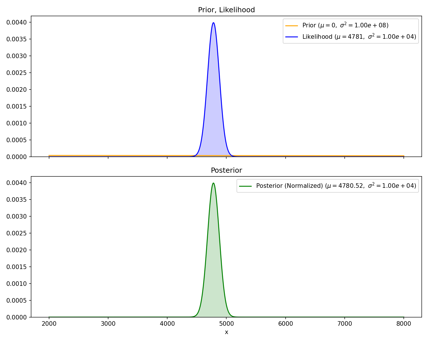
        <p>I’ll note a few things. First, the prior is hard to see
        because it is pretty close to a flat line right around 0.
        Second, the mean of the posterior is very slightly less than the
        measurement. This is because our prior is centered at zero, so
        it will still “pull” the posterior towards it, no matter how
        flat it is. Third, the equation for the standard deviation,
        <math display="inline" xmlns="http://www.w3.org/1998/Math/MathML"><semantics><mi>σ</mi><annotation encoding="application/x-tex">\sigma</annotation></semantics></math>, above guarantees that
        the variance of the posterior is less than or equal to the
        variance of prior and likelihood Gaussians.</p>
        <h3
        id="act-2-multiple-measurements-of-a-stationary-submarine">Act
        2: Multiple Measurements of A Stationary Submarine</h3>
        <p>Now, we get a second measurement,</p>
        <pre xml:space="preserve"><code>   🛥️ ···))·····))     🛥️
&lt;───┼───────────────────┼───&gt; x
    0                  ❓</code></pre>
        <!-- truth: 4900 meters -->
        <table>
        <thead>
        <tr>
        <th style="text-align: left;">Measurement</th>
        <th style="text-align: center;">Range</th>
        </tr>
        </thead>
        <tbody>
        <tr>
        <td style="text-align: left;">#2</td>
        <td style="text-align: center;">4952 meters</td>
        </tr>
        </tbody>
        </table>
        <p>And we’d like to update our probability distribution of the
        other submarine’s position, <math display="inline" xmlns="http://www.w3.org/1998/Math/MathML"><semantics><mrow><msub><mi>f</mi><mi>X</mi></msub><mo stretchy="false" form="prefix">(</mo><mi>x</mi><mo stretchy="false" form="postfix">)</mo></mrow><annotation encoding="application/x-tex">f_X(x)</annotation></semantics></math>. Recalling the math recap from
        the beginning, we can use the posterior from Act 1 as our new
        prior, rinse and repeat.</p>
        <p><math display="block" xmlns="http://www.w3.org/1998/Math/MathML"><semantics><mrow><mtext mathvariant="normal">Act 2 posterior</mtext><mo>=</mo><mfrac><mrow><mtable><mtr><mtd columnalign="center" style="text-align: center"><mtext mathvariant="normal">measurement
 #2</mtext></mtd></mtr><mtr><mtd columnalign="center" style="text-align: center"><mtext mathvariant="normal">likelihood</mtext></mtd></mtr></mtable><mo>×</mo><mtext mathvariant="normal">Act 1
 posterior</mtext></mrow><mtable><mtr><mtd columnalign="center" style="text-align: center"><mrow><mtext mathvariant="normal">probability
 of measurement #2 </mtext><mspace width="0.333em"></mspace></mrow></mtd></mtr><mtr><mtd columnalign="center" style="text-align: center"><mtext mathvariant="normal">across all possible x</mtext></mtd></mtr></mtable></mfrac></mrow><annotation encoding="application/x-tex">\text{Act 2 posterior} = \frac{\substack{{\text{measurement
        \#2}}\\
        {\text{likelihood}}} \times \text{Act 1
        posterior}}{\substack{\text{probability
        of measurement \#2 }\\{\text{across all possible x}}}}</annotation></semantics></math></p>
        <figure>
        <img src="/resources/particle-filter/problem-2.png" alt="problem-2" />
        </figure>
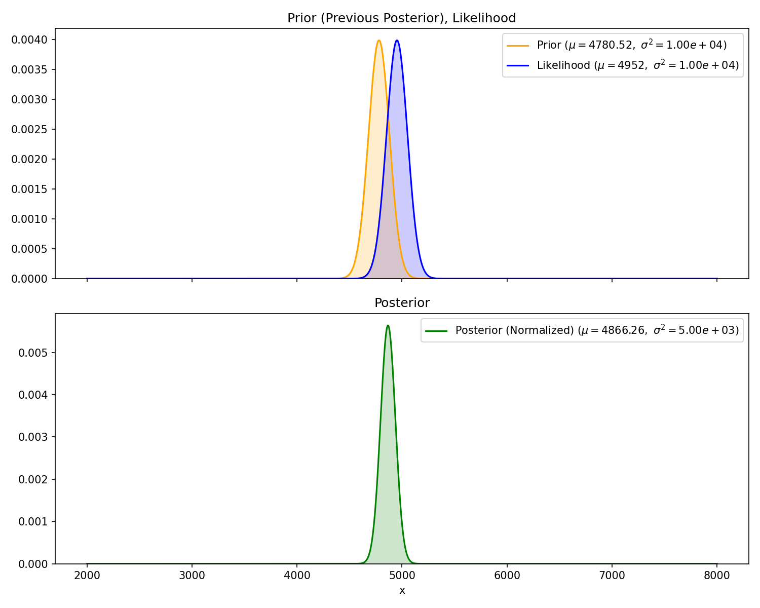
        <p>Again, the variance of the posterior is smaller than the two
        inputs. Since the variance of the prior and likelihood are
        roughly the same, the mean of the posterior is half way in
        between the two.</p>
        <p>One of the powers of Bayesian inference is that it allows
        subjective priors. By that, I mean your domain knowledge and
        lived experience may give you a hunch that the other sub likes
        to hang out in some area and is therefore probably some distance
        away. Bayesian inference allows you to turn this “hunch” into a
        prior. This is possible because (in theory) no matter what prior
        you choose (so long as it is not zero where it matters) with
        enough measurement updates eventually your posterior will
        converge on the true distribution. Therefore we can leverage
        subjective “hunches” while maintaining some mathematical
        guarantees.</p>
        <h3 id="act-3-multiple-measurements-of-a-moving-submarine">Act
        3: Multiple Measurements of a Moving Submarine</h3>
        <p>Now, the other submarine is moving, but we don’t know how
        fast. We take sequential sensor measurements. Our goal is to
        estimate (at the time of the last measurement) the velocity and
        range of the other submarine. We’ll make the following
        assumptions</p>
        <pre xml:space="preserve"><code>   🛥️ ···))······))    🛥️💨
&lt;───┼───────────────────┼───&gt; x
    0                  ❓</code></pre>
        <ul>
        <li>Everything is still in one dimension</li>
        <li>The other sub is moving at a constant velocity</li>
        <li>Our prior on the other submarine’s velocity is <math display="inline" xmlns="http://www.w3.org/1998/Math/MathML"><semantics><mrow><mi>𝒩</mi><mo stretchy="false" form="prefix">(</mo><mi>μ</mi><mo>=</mo><mn>0</mn><mo>,</mo><msup><mi>σ</mi><mn>2</mn></msup><mo>=</mo><mn>5</mn><mo stretchy="false" form="postfix">)</mo></mrow><annotation encoding="application/x-tex">\mathcal{N}(\mu=0,
        \sigma^2=5)</annotation></semantics></math> where a negative value means it is getting
        closer.</li>
        </ul>
        <p>The state of the other submarine is now a random vector <math display="inline" xmlns="http://www.w3.org/1998/Math/MathML"><semantics><mi>X</mi><annotation encoding="application/x-tex">X</annotation></semantics></math>:</p>
        <p><math display="block" xmlns="http://www.w3.org/1998/Math/MathML"><semantics><mrow><mi>x</mi><mo>=</mo><mrow><mo stretchy="true" form="prefix">[</mo><mtable><mtr><mtd columnalign="center" style="text-align: center"><msub><mi>x</mi><mn>1</mn></msub></mtd></mtr><mtr><mtd columnalign="center" style="text-align: center"><msub><mi>x</mi><mn>2</mn></msub></mtd></mtr></mtable><mo stretchy="true" form="postfix">]</mo></mrow><mo>=</mo><mrow><mo stretchy="true" form="prefix">[</mo><mtable><mtr><mtd columnalign="center" style="text-align: center"><mtext mathvariant="normal">position</mtext></mtd></mtr><mtr><mtd columnalign="center" style="text-align: center"><mtext mathvariant="normal">velocity</mtext></mtd></mtr></mtable><mo stretchy="true" form="postfix">]</mo></mrow></mrow><annotation encoding="application/x-tex">x= \begin{bmatrix} x_1 \\ x_2 \end{bmatrix}= \begin{bmatrix}
        \text{position}
        \\ \text{velocity} \end{bmatrix}</annotation></semantics></math></p>
        <p>And its probability distribution is now multivariate Gaussian
        <math display="inline" xmlns="http://www.w3.org/1998/Math/MathML"><semantics><mrow><mi>X</mi><mo>∼</mo><mi>𝒩</mi><mo stretchy="false" form="prefix">(</mo><mi>μ</mi><mo>,</mo><mi mathvariant="normal">Σ</mi><mo stretchy="false" form="postfix">)</mo></mrow><annotation encoding="application/x-tex">X\sim\mathcal{N}(\mu,\Sigma)</annotation></semantics></math>.
        Our prior is</p>
        <p><math display="block" xmlns="http://www.w3.org/1998/Math/MathML"><semantics><mrow><mi>μ</mi><mo>=</mo><mrow><mo stretchy="true" form="prefix">[</mo><mtable><mtr><mtd columnalign="center" style="text-align: center"><mn>0</mn></mtd></mtr><mtr><mtd columnalign="center" style="text-align: center"><mn>0</mn></mtd></mtr></mtable><mo stretchy="true" form="postfix">]</mo></mrow><mo>,</mo><mspace width="1.0em"></mspace><mi mathvariant="normal">Σ</mi><mo>=</mo><mrow><mo stretchy="true" form="prefix">[</mo><mtable><mtr><mtd columnalign="center" style="text-align: center"><msup><mn>10</mn><mn>8</mn></msup></mtd><mtd columnalign="center" style="text-align: center"><mn>0</mn></mtd></mtr><mtr><mtd columnalign="center" style="text-align: center"><mn>0</mn></mtd><mtd columnalign="center" style="text-align: center"><mn>5</mn></mtd></mtr></mtable><mo stretchy="true" form="postfix">]</mo></mrow></mrow><annotation encoding="application/x-tex">\mu =\begin{bmatrix} 0 \\ 0 \end{bmatrix}, \quad
        \Sigma=\begin{bmatrix} 10^8
        &amp; 0 \\ 0 &amp; 5 \end{bmatrix}</annotation></semantics></math></p>
        <p>Again, we will employ Bayesian inference. The problem is now
        two dimensions, but conceptually the technique is the same. We
        will treat the first measurement just as we did in Act 2.
        However, after calculating the posterior <math display="inline" xmlns="http://www.w3.org/1998/Math/MathML"><semantics><mrow><msub><mi>f</mi><mi>X</mi></msub><mo stretchy="false" form="prefix">(</mo><mi>x</mi><mo stretchy="false" form="postfix">)</mo></mrow><annotation encoding="application/x-tex">f_X(x)</annotation></semantics></math> of the random vector, instead
        of immediately turning it into our next prior, we first must
        update it with time. To do this, we need something called a
        “motion model” or “state update equation”. Given a state at
        <math display="inline" xmlns="http://www.w3.org/1998/Math/MathML"><semantics><mrow><mi>t</mi><mo>−</mo><mn>1</mn></mrow><annotation encoding="application/x-tex">t-1</annotation></semantics></math>, and our assumption of
        constant velocity, the state at <math display="inline" xmlns="http://www.w3.org/1998/Math/MathML"><semantics><mi>t</mi><annotation encoding="application/x-tex">t</annotation></semantics></math> is given by</p>
        <p><math display="block" xmlns="http://www.w3.org/1998/Math/MathML"><semantics><mtable><mtr><mtd columnalign="right" style="text-align: right; padding-right: 0"><msub><mtext mathvariant="normal">pos</mtext><mi>t</mi></msub></mtd><mtd columnalign="left" style="text-align: left; padding-left: 0"><mo>=</mo><msub><mtext mathvariant="normal">pos</mtext><mrow><mi>t</mi><mo>−</mo><mn>1</mn></mrow></msub><mo>+</mo><msub><mtext mathvariant="normal">vel</mtext><mrow><mi>t</mi><mo>−</mo><mn>1</mn></mrow></msub><mi mathvariant="normal">Δ</mi><mi>t</mi></mtd></mtr><mtr><mtd columnalign="right" style="text-align: right; padding-right: 0"><msub><mtext mathvariant="normal">vel</mtext><mi>t</mi></msub></mtd><mtd columnalign="left" style="text-align: left; padding-left: 0"><mo>=</mo><msub><mtext mathvariant="normal">vel</mtext><mrow><mi>t</mi><mo>−</mo><mn>1</mn></mrow></msub></mtd></mtr></mtable><annotation encoding="application/x-tex">\begin{aligned}
        \textrm{pos}_t&amp;=\textrm{pos}_{t-1}+\text{vel}_{t-1}\Delta t \\
        \textrm{vel}_t&amp;=\textrm{vel}_{t-1}
        \end{aligned}</annotation></semantics></math></p>
        <p>where <math display="inline" xmlns="http://www.w3.org/1998/Math/MathML"><semantics><mrow><mi mathvariant="normal">Δ</mi><mi>t</mi></mrow><annotation encoding="application/x-tex">\Delta t</annotation></semantics></math> is the time
        in between each sensor reading. This is a linear transformation
        we can write in matrix form:</p>
        <p><math display="block" xmlns="http://www.w3.org/1998/Math/MathML"><semantics><mrow><msub><mrow><mo stretchy="true" form="prefix">[</mo><mtable><mtr><mtd columnalign="center" style="text-align: center"><mtext mathvariant="normal">pos</mtext></mtd></mtr><mtr><mtd columnalign="center" style="text-align: center"><mtext mathvariant="normal">vel</mtext></mtd></mtr></mtable><mo stretchy="true" form="postfix">]</mo></mrow><mi>t</mi></msub><mo>=</mo><mrow><mo stretchy="true" form="prefix">[</mo><mtable><mtr><mtd columnalign="center" style="text-align: center"><mn>1</mn></mtd><mtd columnalign="center" style="text-align: center"><mi mathvariant="normal">Δ</mi><mi>t</mi></mtd></mtr><mtr><mtd columnalign="center" style="text-align: center"><mn>0</mn></mtd><mtd columnalign="center" style="text-align: center"><mn>1</mn></mtd></mtr></mtable><mo stretchy="true" form="postfix">]</mo></mrow><msub><mrow><mo stretchy="true" form="prefix">[</mo><mtable><mtr><mtd columnalign="center" style="text-align: center"><mtext mathvariant="normal">pos</mtext></mtd></mtr><mtr><mtd columnalign="center" style="text-align: center"><mtext mathvariant="normal">vel</mtext></mtd></mtr></mtable><mo stretchy="true" form="postfix">]</mo></mrow><mrow><mi>t</mi><mo>−</mo><mn>1</mn></mrow></msub><mo>=</mo><mi>A</mi><msub><mrow><mo stretchy="true" form="prefix">[</mo><mtable><mtr><mtd columnalign="center" style="text-align: center"><mtext mathvariant="normal">pos</mtext></mtd></mtr><mtr><mtd columnalign="center" style="text-align: center"><mtext mathvariant="normal">vel</mtext></mtd></mtr></mtable><mo stretchy="true" form="postfix">]</mo></mrow><mrow><mi>t</mi><mo>−</mo><mn>1</mn></mrow></msub></mrow><annotation encoding="application/x-tex">\begin{bmatrix} \text{pos} \\ \text{vel} \end{bmatrix}_t =
        \begin{bmatrix} 1
        &amp; \Delta t \\ 0 &amp; 1 \end{bmatrix} \begin{bmatrix}
        \text{pos} \\ \text{vel}
        \end{bmatrix}_{t-1} = A \begin{bmatrix} \text{pos} \\ \text{vel}
        \end{bmatrix}_{t-1}</annotation></semantics></math></p>
        <p>(I’m sticking with convention here to call this matrix <math display="inline" xmlns="http://www.w3.org/1998/Math/MathML"><semantics><mi>A</mi><annotation encoding="application/x-tex">A</annotation></semantics></math>).</p>
        <p>Given a state vector we can transform it with time, but how
        do we transform a continuous distribution? Let’s change our
        framing slightly; instead of thinking about probability
        distributions, let’s consider the random variable <math display="inline" xmlns="http://www.w3.org/1998/Math/MathML"><semantics><mrow><mi>X</mi><mo>=</mo><mo stretchy="false" form="prefix">{</mo><mtext mathvariant="normal">pos</mtext><mo>,</mo><mtext mathvariant="normal">vel</mtext><mo stretchy="false" form="postfix">}</mo></mrow><annotation encoding="application/x-tex">X=\{\text{pos},\text{vel}\}</annotation></semantics></math> which
        this distribution describes. Again, we are fortunate that our
        variable is Gaussian. Thinking back to an intro stats class, you
        may remember that multiplying a random variable by a constant
        <math display="inline" xmlns="http://www.w3.org/1998/Math/MathML"><semantics><mi>b</mi><annotation encoding="application/x-tex">b</annotation></semantics></math> scales its mean by <math display="inline" xmlns="http://www.w3.org/1998/Math/MathML"><semantics><mi>b</mi><annotation encoding="application/x-tex">b</annotation></semantics></math> and its variance by <math display="inline" xmlns="http://www.w3.org/1998/Math/MathML"><semantics><msup><mi>b</mi><mn>2</mn></msup><annotation encoding="application/x-tex">b^2</annotation></semantics></math>. This extends to random vectors.
        Given any linear transformation <math display="inline" xmlns="http://www.w3.org/1998/Math/MathML"><semantics><mrow><mi>Y</mi><mo>=</mo><mi>B</mi><mi>X</mi></mrow><annotation encoding="application/x-tex">Y=BX</annotation></semantics></math>,</p>
        <p><math display="block" xmlns="http://www.w3.org/1998/Math/MathML"><semantics><mrow><mi>E</mi><mo stretchy="false" form="prefix">[</mo><mi>Y</mi><mo stretchy="false" form="postfix">]</mo><mo>=</mo><mi>B</mi><mi>E</mi><mo stretchy="false" form="prefix">[</mo><mi>X</mi><mo stretchy="false" form="postfix">]</mo></mrow><annotation encoding="application/x-tex">E[Y]=B E[X]</annotation></semantics></math></p>
        <p><math display="block" xmlns="http://www.w3.org/1998/Math/MathML"><semantics><mrow><mi>C</mi><mi>o</mi><mi>v</mi><mo stretchy="false" form="prefix">(</mo><mi>Y</mi><mo stretchy="false" form="postfix">)</mo><mo>=</mo><mi>B</mi><mi>C</mi><mi>o</mi><mi>v</mi><mo stretchy="false" form="prefix">(</mo><mi>X</mi><mo stretchy="false" form="postfix">)</mo><msup><mi>B</mi><mi>T</mi></msup></mrow><annotation encoding="application/x-tex">Cov(Y)=B Cov(X)B^T</annotation></semantics></math></p>
        <p>Because the Gaussian distribution is defined by this mean and
        variance, the resulting distribution of our random variable is
        also Gaussian with</p>
        <p><math display="block" xmlns="http://www.w3.org/1998/Math/MathML"><semantics><mrow><mi>𝒩</mi><mo stretchy="false" form="prefix">(</mo><mi>μ</mi><mo>,</mo><mi mathvariant="normal">Σ</mi><mo stretchy="false" form="postfix">)</mo><mo>→</mo><mi>𝒩</mi><mo stretchy="false" form="prefix">(</mo><mi>A</mi><mi>μ</mi><mo>,</mo><mi>A</mi><mi mathvariant="normal">Σ</mi><msup><mi>A</mi><mi>T</mi></msup><mo stretchy="false" form="postfix">)</mo></mrow><annotation encoding="application/x-tex">\mathcal{N}(\mu,\Sigma)\to
        \mathcal{N}(A\mu,A\Sigma A^T)</annotation></semantics></math></p>
        <p>So long as our motion model is a linear transformation and
        our prior and measurements are still Gaussian, the posterior
        will remain Gaussian, and therefore the entire process can be
        solved analytically. Say we receive the following three
        measurements:</p>
        <table>
        <thead>
        <tr>
        <th style="text-align: left;">Measurement</th>
        <th style="text-align: center;">Time</th>
        <th style="text-align: center;">Range</th>
        </tr>
        </thead>
        <tbody>
        <tr>
        <td style="text-align: left;">#1</td>
        <td style="text-align: center;">0 seconds</td>
        <td style="text-align: center;">7507 meters</td>
        </tr>
        <tr>
        <td style="text-align: left;">#2</td>
        <td style="text-align: center;">60 seconds</td>
        <td style="text-align: center;">7671 meters</td>
        </tr>
        <tr>
        <td style="text-align: left;">#3</td>
        <td style="text-align: center;">200 seconds</td>
        <td style="text-align: center;">8099 meters</td>
        </tr>
        </tbody>
        </table>
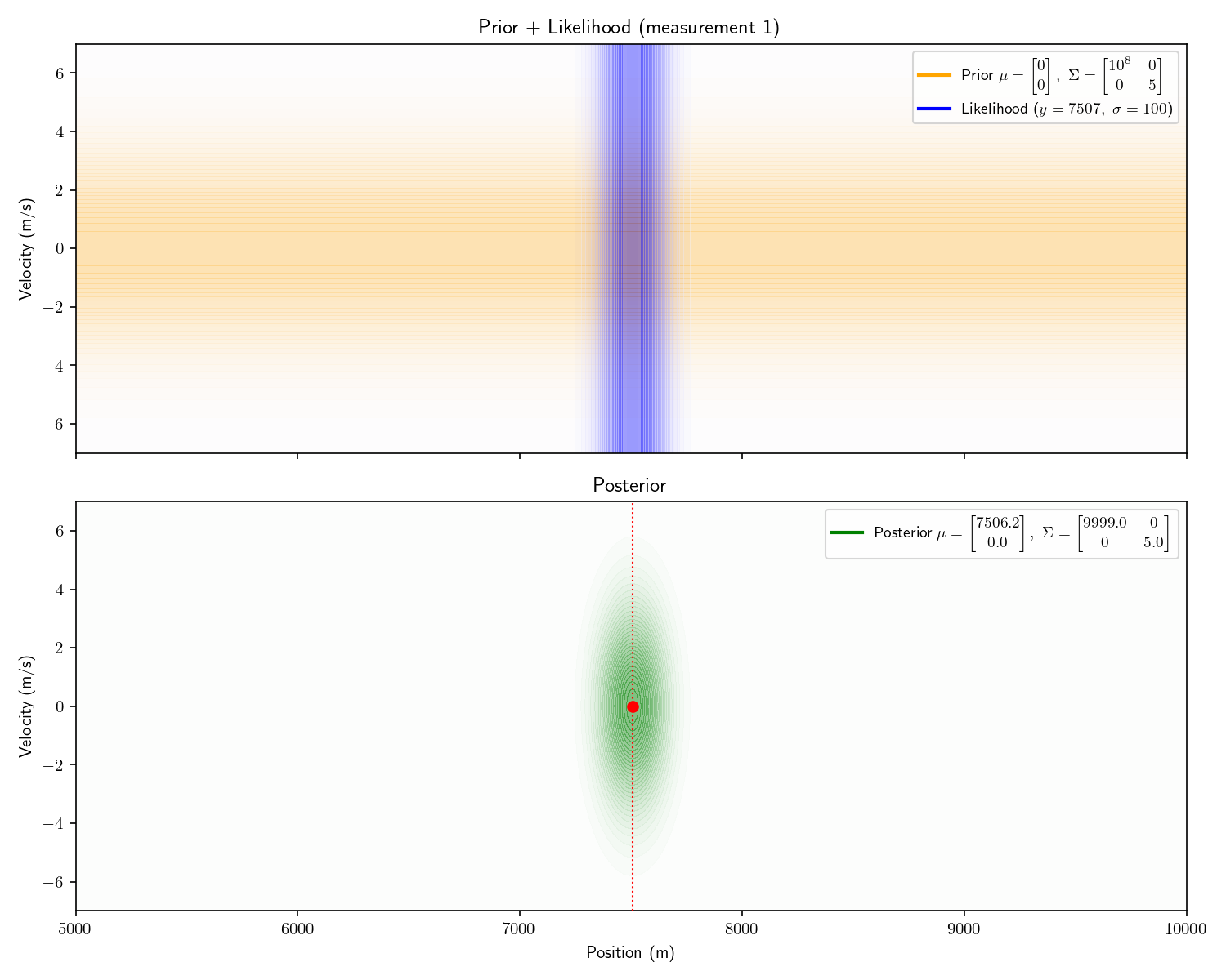
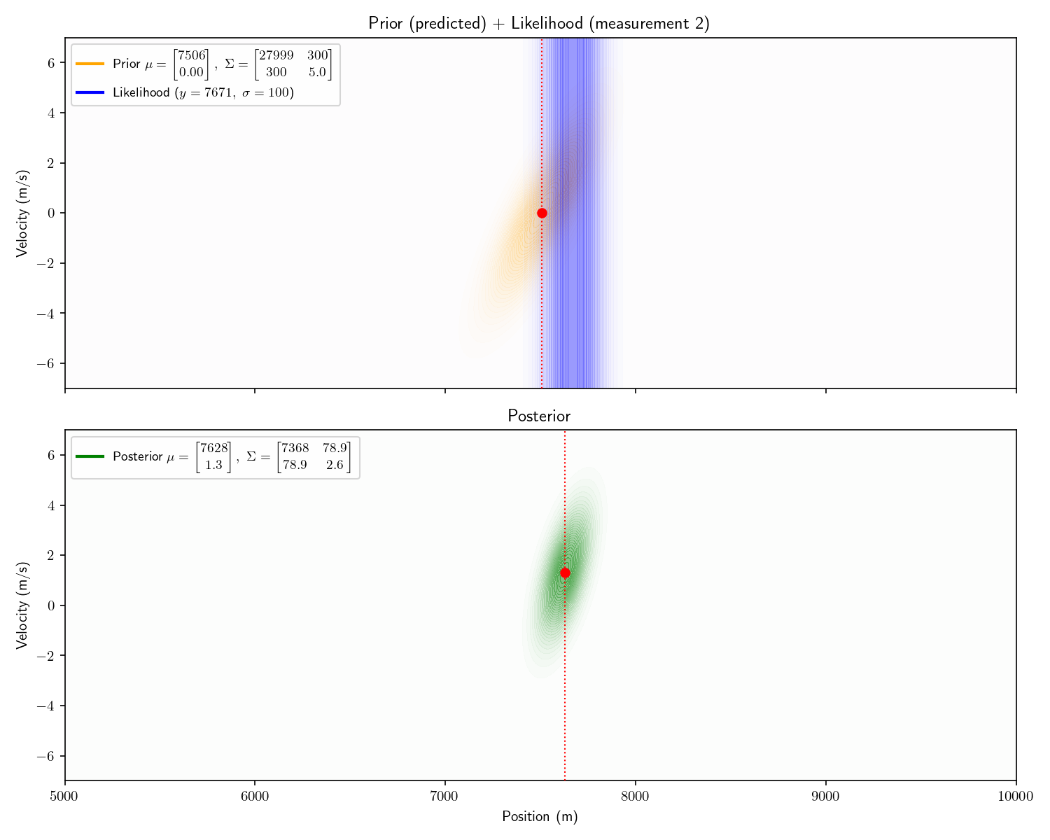
        <p>To process the first, we apply Bayes’ theorem just as we did
        in Act 2. I’ve plotted top-down heatmaps of our probability
        distributions. Getting oriented, an informationless prior would
        look like a uniform, light orange background. Our prior is a bit
        better than informationless: we know the velocity is probably
        between <math display="inline" xmlns="http://www.w3.org/1998/Math/MathML"><semantics><mrow><mi>±</mi><mn>4</mn></mrow><annotation encoding="application/x-tex">\pm 4</annotation></semantics></math> m/s.</p>
        <p>Our sensor still provides only range information. Therefore
        it appears as a 1D Gaussian smeared uniformly across the
        velocity axis.</p>
        <figure>
        <img src="/resources/particle-filter/problem-3-meas-1.png" alt="problem-3-meas-1" />
        </figure>
        <blockquote>
        <p><em>Aside: I haven’t plotted the actual prior here – it would
        appear as a single color. I’ve emphasized things for visual
        effect.</em></p>
        </blockquote>
        <p>Notice how the posterior mean is slightly lower than 7507.
        This is because our prior is not truly “informationless” it is
        just a very flat Gaussian centered at 0, so it will pull the
        posterior slightly towards 0.</p>
        <figure>
        <img src="/resources/particle-filter/problem-3-meas-2.png" alt="problem-3-meas-2" />
        </figure>
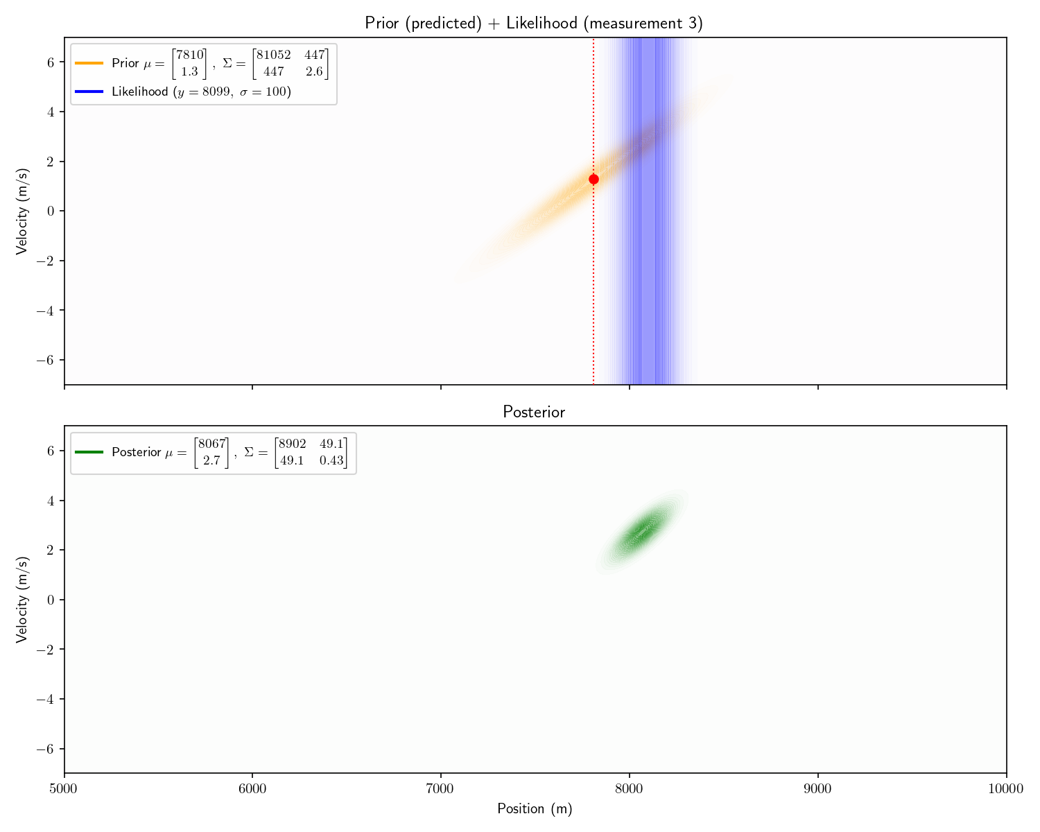
        <figure>
        <img src="/resources/particle-filter/problem-3-meas-3.png" alt="problem-3-meas-3" />
        </figure>
        <blockquote>
        <p>Aside: the first posterior’s covariance matrix has 0s in its
        off diagonals. This is a fancy way of pointing out that it isn’t
        slanted. After we apply the motion model, these off-diagonal
        elements become non-zero and it becomes slanted. It is this
        covariance matrix that carries the “information” about the
        relationship between the possible positions and velocities:
        i.e., “If the sub has a positive velocity it is probably further
        away now”.</p>
        </blockquote>
        <p>Let’s zoom out for one moment. Our goal is to motivate the
        particle filter. Until this point we haven’t defined
        <em>“particle”</em> or <em>“filter”</em>. The approach I’ve just
        described is is called <em>“recursive Bayesian estimation”</em>
        or a <em>“Bayesian Filter”</em>. The first phrase describes
        exactly what we’ve done: recursively apply Bayes’ theorem to
        estimate the state of the submarine. As for the latter,
        <em>“filtering”</em> simply means we are estimating the state of
        the submarine at the time of the last measurement as opposed to
        during the whole encounter. At this point you know literally 1/2
        of <em>“particle filter”</em>, and our conceptual understanding
        is roughly half way there as well.</p>
        <p>In particular, a Bayesian filter where the prior and
        measurements are Gaussian and the state update is linear is
        called a <em>“Kalman Filter”</em>.</p>
        <p>Notice one more thing about our results. Our final posterior
        tells us that the other submarine’s velocity is between +2 and
        +4. This is remarkable because we never received any information
        about its velocity! We call velocity a “hidden state” because it
        is never observed. One powerful trait of Kalman Filters is that
        they can provide estimates of states which are never
        observed.</p>
        <blockquote>
        <p><em>Aside: the Kalman filter can also represent Gaussian
        noise in the state update. For example, imagine the velocity of
        the submarine depended on the temperature/salinity of the water.
        We could model the effect of this unknown environment as
        Gaussian noise (just like we did with the
        measurements).</em></p>
        </blockquote>
        <blockquote>
        <p><em>Aside: the “extended Kalman filter” (EKF) can use any
        differentiable function for the state-transition model (rather
        than linear). This involves constructing a Jacobian (matrix of
        partial derivatives) to update the covariance with. The EKF is
        the de facto technique of GPS systems.</em></p>
        </blockquote>
        <h3 id="act-4-histogram-filter">Act 4: Histogram Filter</h3>
        <p>Now imagine that before receiving the first sensor report, we
        receive an intelligence that the other submarine is between
        4,600 and 6,000 meters away.</p>
        <pre xml:space="preserve"><code>   🛥️ ···))······))       🛥️
&lt;───┼────────────────┼──────────┼───&gt; x
0                  4,600  ❓  6,000</code></pre>
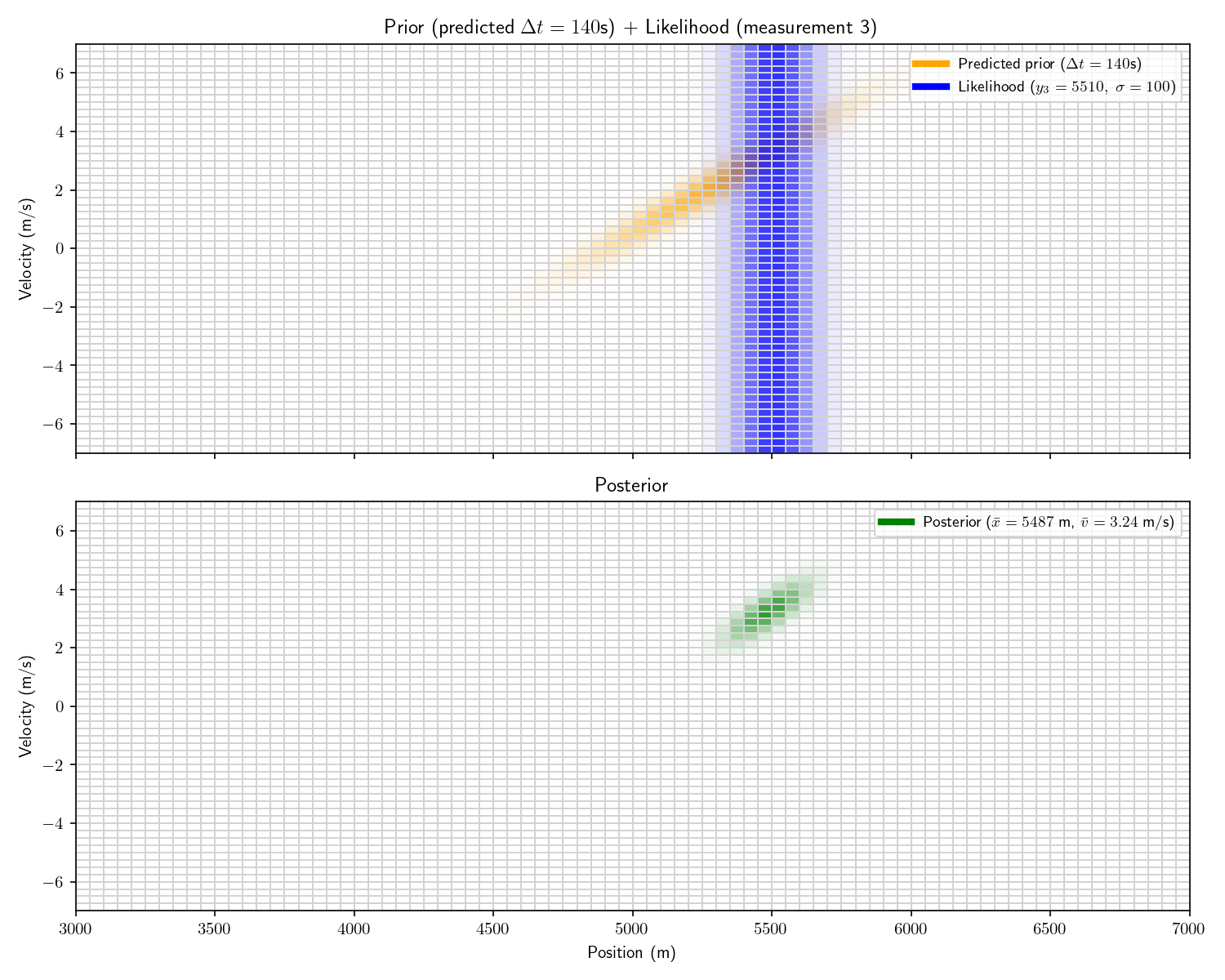
        <p>And then we receive the following three measurements:</p>
        <table>
        <thead>
        <tr>
        <th style="text-align: left;">Measurement</th>
        <th style="text-align: center;">Time</th>
        <th style="text-align: center;">Range</th>
        </tr>
        </thead>
        <tbody>
        <tr>
        <td style="text-align: left;">#1</td>
        <td style="text-align: center;">0 seconds</td>
        <td style="text-align: center;">4781 meters</td>
        </tr>
        <tr>
        <td style="text-align: left;">#2</td>
        <td style="text-align: center;">60 seconds</td>
        <td style="text-align: center;">5063 meters</td>
        </tr>
        <tr>
        <td style="text-align: left;">#3</td>
        <td style="text-align: center;">200 seconds</td>
        <td style="text-align: center;">5510 meters</td>
        </tr>
        </tbody>
        </table>
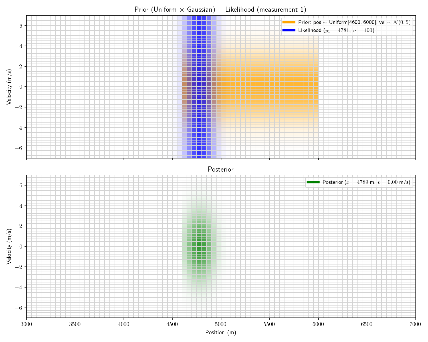
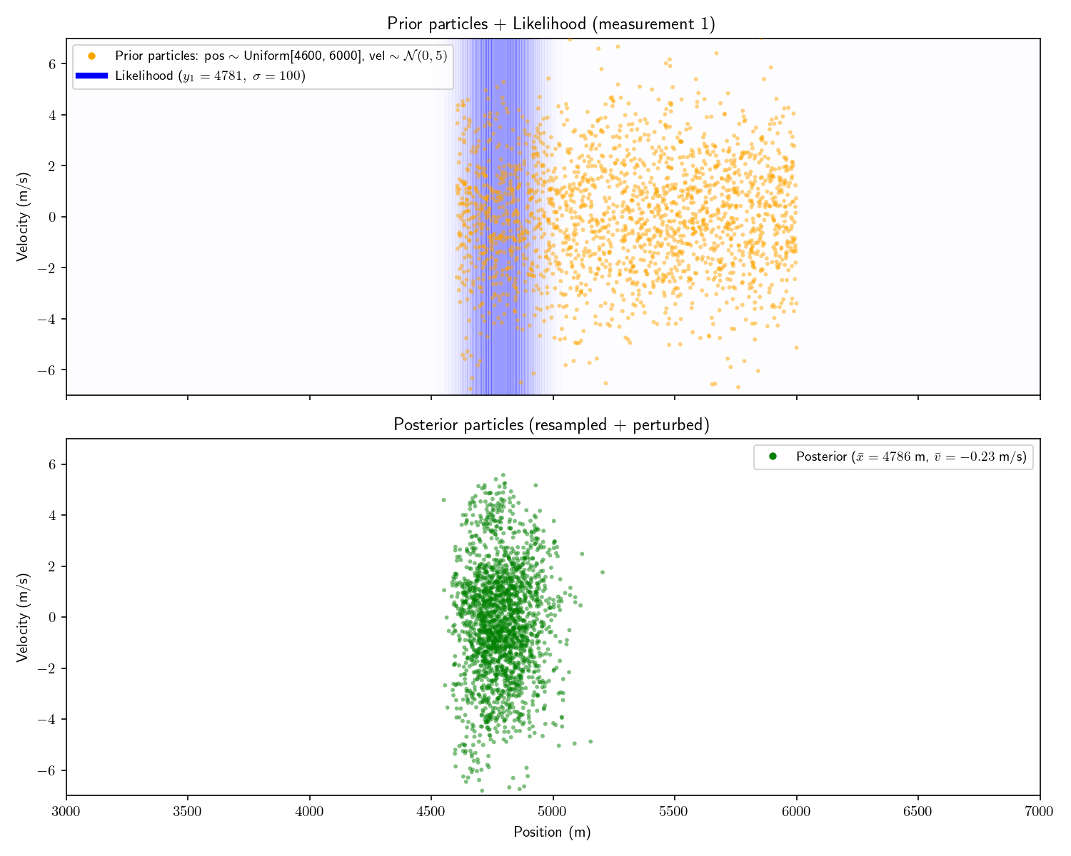
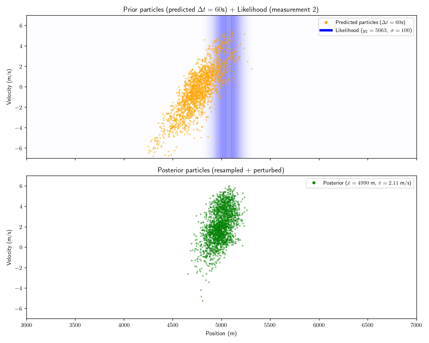
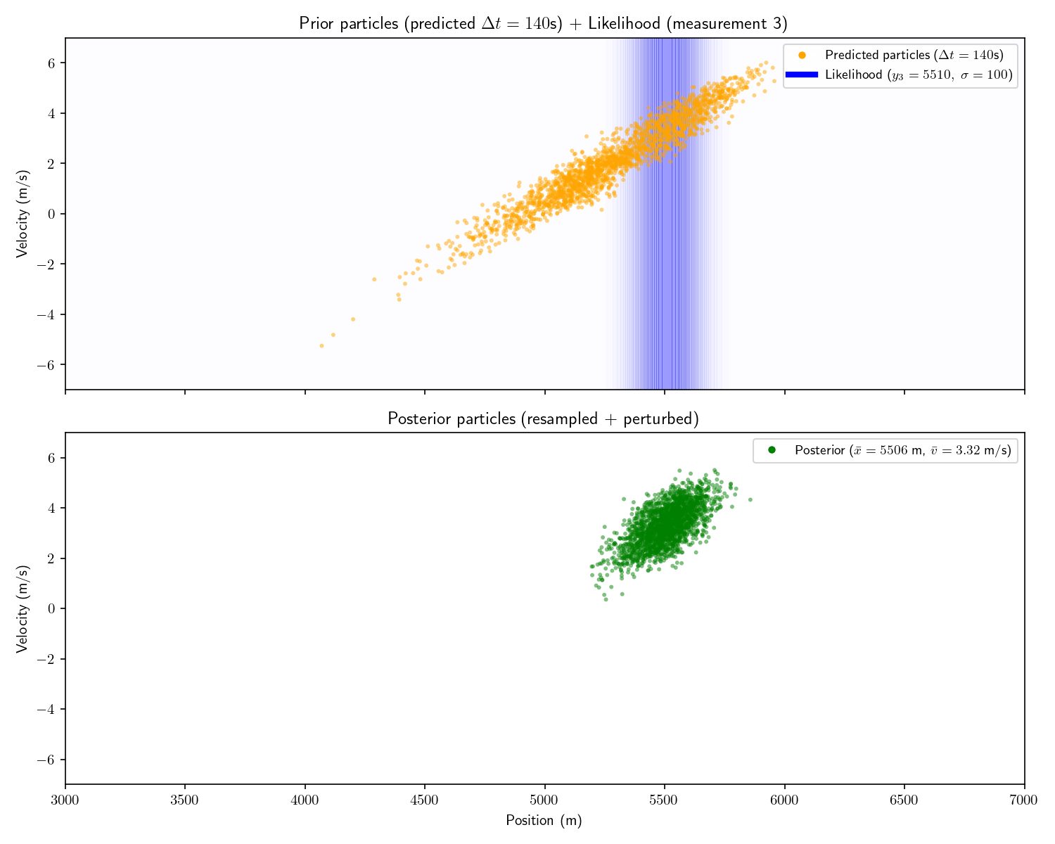
        <p>We can incorporate the intelligence report into our Bayesian
        framework as a uniform prior:</p>
        <p><math display="block" xmlns="http://www.w3.org/1998/Math/MathML"><semantics><mrow><msub><mi>f</mi><mi>X</mi></msub><mo stretchy="false" form="prefix">(</mo><mi>x</mi><mo stretchy="false" form="postfix">)</mo><mo>=</mo><mfrac><mn>1</mn><mtext mathvariant="normal">1,400</mtext></mfrac><mspace width="1.0em"></mspace><mrow><mtext mathvariant="normal">for </mtext><mspace width="0.333em"></mspace></mrow><mi>x</mi><mo>∈</mo><mo stretchy="false" form="prefix">[</mo><mtext mathvariant="normal">4,600</mtext><mo>,</mo><mtext mathvariant="normal">6,000</mtext><mo stretchy="false" form="postfix">]</mo></mrow><annotation encoding="application/x-tex">f_X(x) = \frac{1}{\text{1,400}} \quad \text{for } x \in
        [\text{4,600},
        \text{6,000}]</annotation></semantics></math></p>
        <p>The problem with a uniform prior is that we can no longer
        solve the problem analytically. What can we do instead? One
        option divide the x-dimension into 200 “bins” then calculate the
        prior and likelihood for each bin. Then, using the same linear
        motion update</p>
        <p><math display="block" xmlns="http://www.w3.org/1998/Math/MathML"><semantics><mrow><msub><mrow><mo stretchy="true" form="prefix">[</mo><mtable><mtr><mtd columnalign="center" style="text-align: center"><mtext mathvariant="normal">pos</mtext></mtd></mtr><mtr><mtd columnalign="center" style="text-align: center"><mtext mathvariant="normal">vel</mtext></mtd></mtr></mtable><mo stretchy="true" form="postfix">]</mo></mrow><mi>t</mi></msub><mo>=</mo><mrow><mo stretchy="true" form="prefix">[</mo><mtable><mtr><mtd columnalign="center" style="text-align: center"><mn>1</mn></mtd><mtd columnalign="center" style="text-align: center"><mi mathvariant="normal">Δ</mi><mi>t</mi></mtd></mtr><mtr><mtd columnalign="center" style="text-align: center"><mn>0</mn></mtd><mtd columnalign="center" style="text-align: center"><mn>1</mn></mtd></mtr></mtable><mo stretchy="true" form="postfix">]</mo></mrow><msub><mrow><mo stretchy="true" form="prefix">[</mo><mtable><mtr><mtd columnalign="center" style="text-align: center"><mtext mathvariant="normal">pos</mtext></mtd></mtr><mtr><mtd columnalign="center" style="text-align: center"><mtext mathvariant="normal">vel</mtext></mtd></mtr></mtable><mo stretchy="true" form="postfix">]</mo></mrow><mrow><mi>t</mi><mo>−</mo><mn>1</mn></mrow></msub><mo>=</mo><mi>A</mi><msub><mrow><mo stretchy="true" form="prefix">[</mo><mtable><mtr><mtd columnalign="center" style="text-align: center"><mtext mathvariant="normal">pos</mtext></mtd></mtr><mtr><mtd columnalign="center" style="text-align: center"><mtext mathvariant="normal">vel</mtext></mtd></mtr></mtable><mo stretchy="true" form="postfix">]</mo></mrow><mrow><mi>t</mi><mo>−</mo><mn>1</mn></mrow></msub></mrow><annotation encoding="application/x-tex">\begin{bmatrix} \text{pos} \\ \text{vel} \end{bmatrix}_t =
        \begin{bmatrix} 1
        &amp; \Delta t \\ 0 &amp; 1 \end{bmatrix} \begin{bmatrix}
        \text{pos} \\ \text{vel}
        \end{bmatrix}_{t-1} = A \begin{bmatrix} \text{pos} \\ \text{vel}
        \end{bmatrix}_{t-1}</annotation></semantics></math></p>
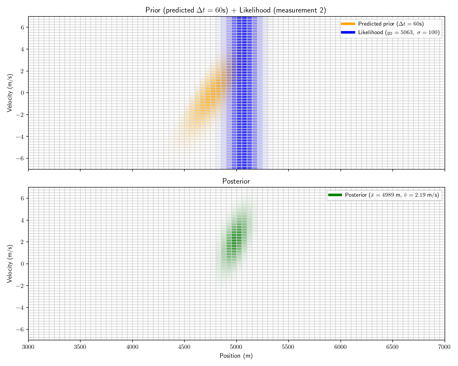
        <p>For each bin in step <math display="inline" xmlns="http://www.w3.org/1998/Math/MathML"><semantics><mrow><mo stretchy="false" form="prefix">(</mo><mi>t</mi><mo>−</mo><mn>1</mn><mo stretchy="false" form="postfix">)</mo></mrow><annotation encoding="application/x-tex">(t-1)</annotation></semantics></math>’s
        posterior, transform its state <math display="inline" xmlns="http://www.w3.org/1998/Math/MathML"><semantics><msub><mi>x</mi><mn>1</mn></msub><annotation encoding="application/x-tex">x_1</annotation></semantics></math> into <math display="inline" xmlns="http://www.w3.org/1998/Math/MathML"><semantics><msub><mi>x</mi><mn>2</mn></msub><annotation encoding="application/x-tex">x_2</annotation></semantics></math> using <math display="inline" xmlns="http://www.w3.org/1998/Math/MathML"><semantics><mi>A</mi><annotation encoding="application/x-tex">A</annotation></semantics></math> and add that probability to step
        <math display="inline" xmlns="http://www.w3.org/1998/Math/MathML"><semantics><mi>t</mi><annotation encoding="application/x-tex">t</annotation></semantics></math>’s prior’s bin at <math display="inline" xmlns="http://www.w3.org/1998/Math/MathML"><semantics><msub><mi>x</mi><mn>2</mn></msub><annotation encoding="application/x-tex">x_2</annotation></semantics></math>.</p>
        <blockquote>
        <p><em>Aside: alternatively we could have used a Gaussian prior
        with (<math display="inline" xmlns="http://www.w3.org/1998/Math/MathML"><semantics><mrow><mi>μ</mi><mo>=</mo><mn>5</mn><mo>,</mo><mn>300</mn><mo>,</mo><mi>σ</mi><mo>=</mo><mn>700</mn><mo stretchy="false" form="postfix">)</mo></mrow><annotation encoding="application/x-tex">\mu=5,300,
        \sigma=700)</annotation></semantics></math>, called it close enough, and used a Kalman
        Filter. This sounds hacky, but it’s often often a good
        option.</em></p>
        </blockquote>
        <figure>
        <img src="/resources/particle-filter/problem-5-meas-1.png" alt="problem-5-meas-1" />
        </figure>
        <figure>
        <img src="/resources/particle-filter/problem-5-meas-2.png" alt="problem-5-meas-2" />
        </figure>
        <figure>
        <img src="/resources/particle-filter/problem-5-meas-3.png" alt="problem-5-meas-3" />
        </figure>
        <p>Let’s take one more step back. What we’ve just constructed is
        called a “Histogram Filter”. Our solution is no longer
        analytical – that is we’ve approximated our continuous
        distributions with a finite grid. This sacrifices some
        precision, but allows us to consider non-Gaussian priors.</p>
        <p>In this Act we used the same motion model <math display="inline" xmlns="http://www.w3.org/1998/Math/MathML"><semantics><mi>A</mi><annotation encoding="application/x-tex">A</annotation></semantics></math> as in Act 3. However, now that
        we’ve abandoned the requirement of an analytical solution, our
        motion model no longer needs to be linear either. So long as we
        can come up with a way to “update” the probability in the
        posterior forward in time, we can do so however we wish. For
        example, say we know that every 10 minutes the other submarine
        turns around. We could have a literal if-else statement in our
        motion update that if <math display="inline" xmlns="http://www.w3.org/1998/Math/MathML"><semantics><mrow><mi>t</mi><mi>%</mi><mo stretchy="false" form="prefix">(</mo><mn>10</mn><mo>*</mo><mn>60</mn><mo stretchy="false" form="postfix">)</mo><mo>=</mo><mo>=</mo><mn>0</mn></mrow><annotation encoding="application/x-tex">t\%(10*60)==0</annotation></semantics></math>, negate the velocity.
        This is impossible with a Kalman Filter.</p>
        <p>Finally, note that while our measurements have remained
        Gaussian they need not have. Once we start solving things
        numerically, we can drop any requirements about functions being
        Gaussian.</p>
        <h3 id="act-5-particle-filter">Act 5: Particle Filter</h3>
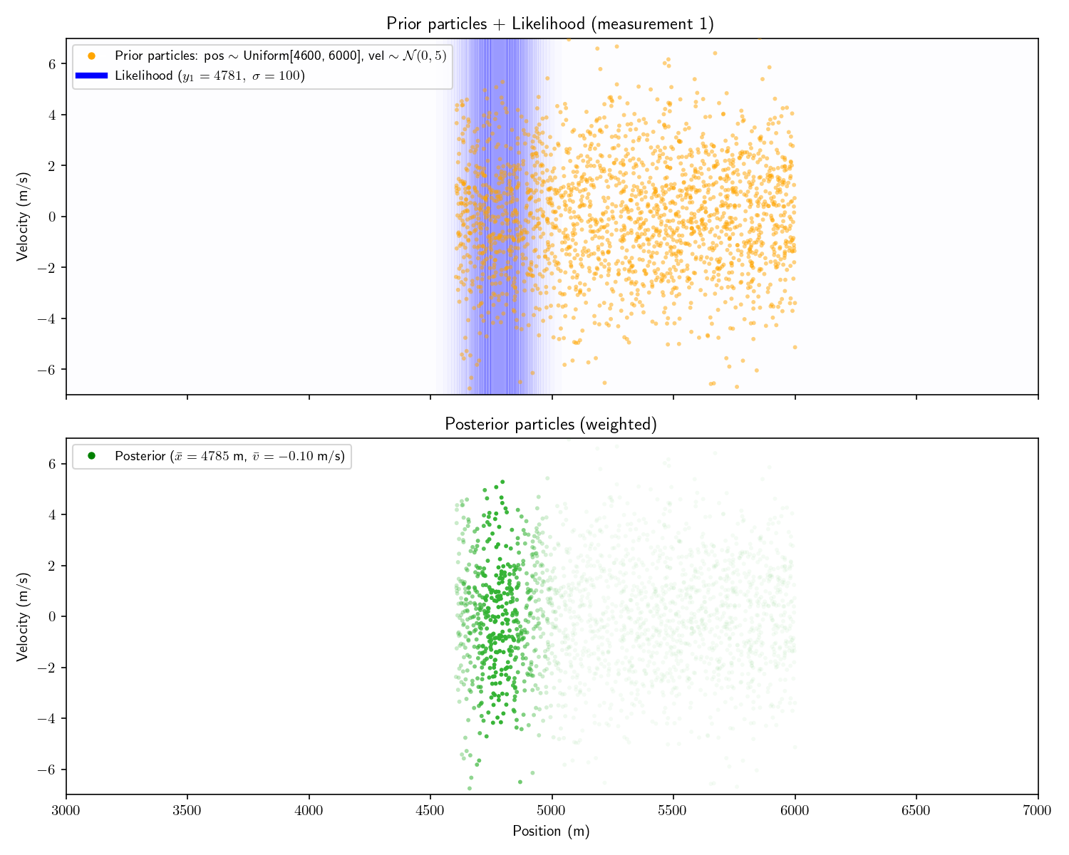
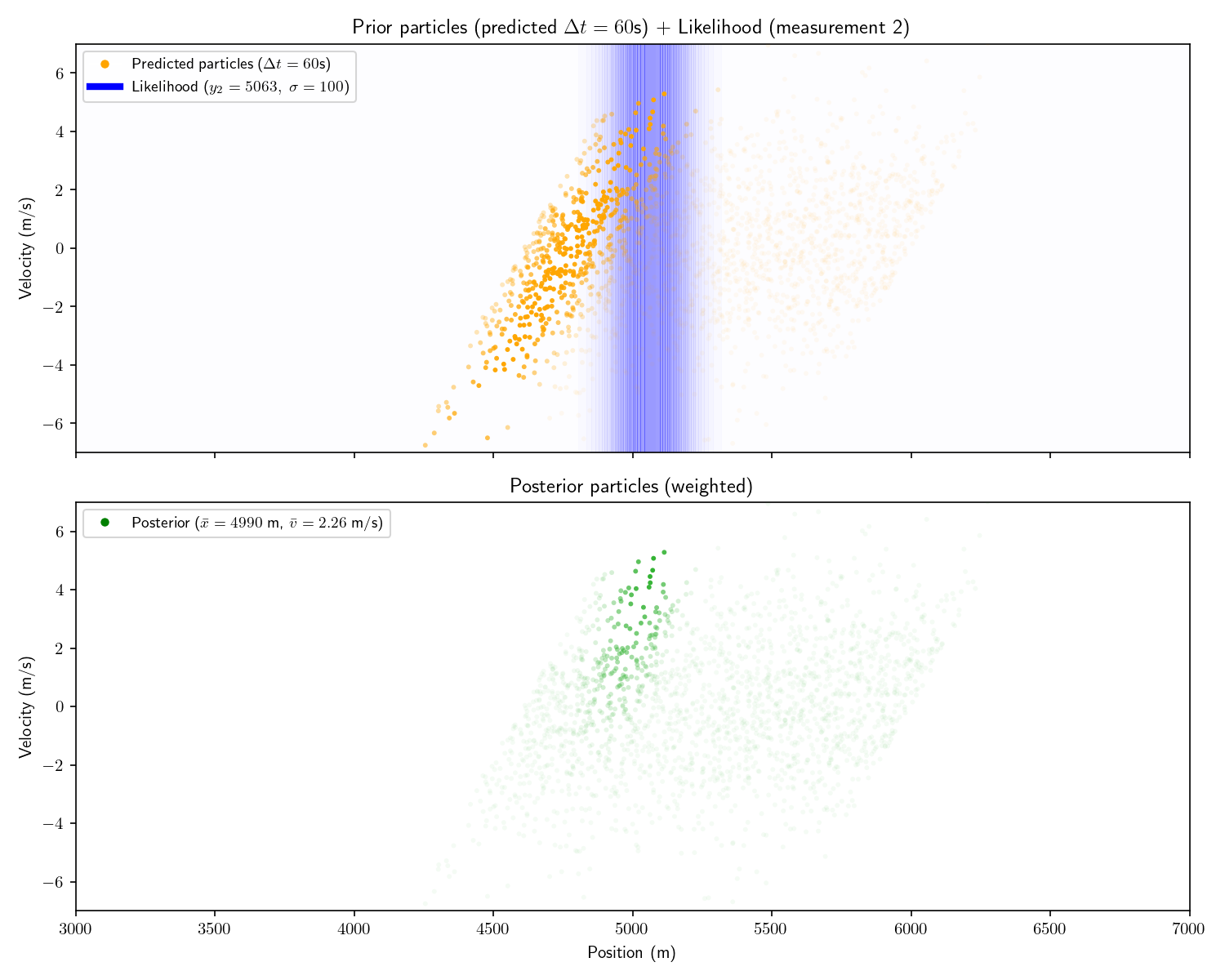
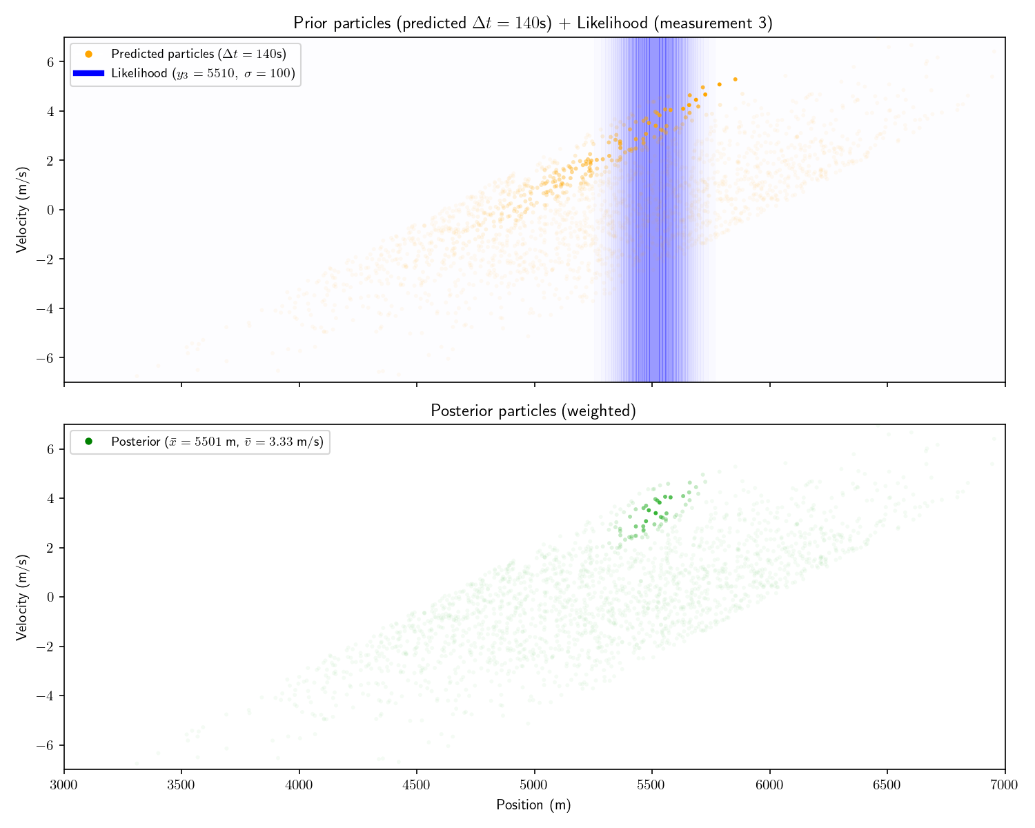
        <p>Now let’s consider a higher-dimensional problem: both
        submarines move in three dimensions. We would like to track both
        position <math display="inline" xmlns="http://www.w3.org/1998/Math/MathML"><semantics><mrow><mo stretchy="false" form="prefix">{</mo><mi>x</mi><mo>,</mo><mi>y</mi><mo>,</mo><mi>z</mi><mo stretchy="false" form="postfix">}</mo></mrow><annotation encoding="application/x-tex">\{x,y,z\}</annotation></semantics></math> and velocity
        <math display="inline" xmlns="http://www.w3.org/1998/Math/MathML"><semantics><mrow><mo stretchy="false" form="prefix">{</mo><msub><mi>v</mi><mi>x</mi></msub><mo>,</mo><msub><mi>v</mi><mi>y</mi></msub><mo>,</mo><msub><mi>v</mi><mi>z</mi></msub><mo stretchy="false" form="postfix">}</mo></mrow><annotation encoding="application/x-tex">\{v_x,v_y,v_z\}</annotation></semantics></math>. Assume our
        measurements are 3d Gaussians on <math display="inline" xmlns="http://www.w3.org/1998/Math/MathML"><semantics><mrow><mo stretchy="false" form="prefix">{</mo><mi>x</mi><mo>,</mo><mi>y</mi><mo>,</mo><mi>z</mi><mo stretchy="false" form="postfix">}</mo></mrow><annotation encoding="application/x-tex">\{x,y,z\}</annotation></semantics></math> and our prior is a uniform
        distribution over a cube in <math display="inline" xmlns="http://www.w3.org/1998/Math/MathML"><semantics><mrow><mo stretchy="false" form="prefix">{</mo><mi>x</mi><mo>,</mo><mi>y</mi><mo>,</mo><mi>z</mi><mo stretchy="false" form="postfix">}</mo></mrow><annotation encoding="application/x-tex">\{x,y,z\}</annotation></semantics></math>.</p>
        <p>If, like before, we split each dimension into 200 bins, we
        now have <math display="inline" xmlns="http://www.w3.org/1998/Math/MathML"><semantics><mrow><msup><mn>200</mn><mn>6</mn></msup><mo>=</mo><mn>64</mn><mspace width="0.278em"></mspace><mtext mathvariant="normal">Trillion</mtext></mrow><annotation encoding="application/x-tex">200^6=64\;\text{Trillion}</annotation></semantics></math> bins. Using
        one float (32 bits) to store each bin’s value would require
        <math display="inline" xmlns="http://www.w3.org/1998/Math/MathML"><semantics><mrow><mn>32</mn><mo>×</mo><mn>64</mn><mo>×</mo><msup><mn>10</mn><mn>12</mn></msup><mspace width="0.278em"></mspace><mtext mathvariant="normal">bits</mtext><mo>≈</mo><mn>250</mn><mspace width="0.278em"></mspace><mtext mathvariant="normal">Terabytes</mtext></mrow><annotation encoding="application/x-tex">32\times 64\times 10^{12}
        \;\text{bits}\approx250\;\text{Terabytes}</annotation></semantics></math>. This is an
        example of “the curse of dimensionality”.</p>
        <p>Let’s think about what’s happening here. In our 2-dimensional
        example, after 3 measurements we are almost certain the other
        submarine has a positive velocity. We nonetheless multiply the
        prior (0) by the likelihood (0) to get the posterior (0) for
        every bin with negative velocity. This is a tremendous waste of
        compute. There are some tricks like having a dynamic
        discretization: have very wide bins where there is no
        probability and very small grids where the probability is
        non-zero. Possible, but adds quite a bit of complexity.</p>
        <p>Note that the Kalman filter does not suffer from the curse of
        dimensionality. Since it only needs to keep track of the mean
        and covariance matrix, which, in 6 dimensions only require 42
        floats.</p>
        <blockquote>
        <p><em>Aside: the idea of assuming a Gaussian distribution to
        avoid the curse of dimensionality is not unique to the Kalman
        Filter. In machine learning, Quadratic Discriminant Analysis and
        Naive Bayes leverage this idea.</em></p>
        </blockquote>
        <p>The particle filter solves this problem. Instead of moving
        our probability between bins, leaving many bins with zero
        probability, why not <em>move the bins themselves</em>? Call
        these moving bins “particles”. Each particle is comprised of its
        state <math display="inline" xmlns="http://www.w3.org/1998/Math/MathML"><semantics><mrow><mo stretchy="false" form="prefix">{</mo><mtext mathvariant="normal">position</mtext><mo>,</mo><mtext mathvariant="normal">velocity</mtext><mo stretchy="false" form="postfix">}</mo></mrow><annotation encoding="application/x-tex">\{\text{position},\text{velocity}\}</annotation></semantics></math>
        and its probability which we call its “weight”.</p>
        <p>To construct our set of particles, sample from the first
        prior distribution. There is no longer a need to discretize our
        likelihood functions as we can evaluate them directly at the
        state of each particle. After applying the likelihood function,
        we update each particle using our state-transition model <math display="inline" xmlns="http://www.w3.org/1998/Math/MathML"><semantics><mi>A</mi><annotation encoding="application/x-tex">A</annotation></semantics></math>. Like the histogram filter, we need
        not use a linear state-transition model or Gaussian
        prior/likelihoods. Note that the superscripts denote the
        particle index, not an exponent. Typically, the subscript is
        reserved for the time index.</p>
        <p><math display="block" xmlns="http://www.w3.org/1998/Math/MathML"><semantics><mrow><mtext mathvariant="normal">particle 1 (state</mtext><mspace width="0.222em"></mspace><msup><mi>x</mi><mn>1</mn></msup><mo stretchy="false" form="postfix">)</mo><mo>:</mo><mspace width="1.0em"></mspace><msubsup><mi>x</mi><mi>t</mi><mn>1</mn></msubsup><mo>=</mo><mrow><mo stretchy="true" form="prefix">[</mo><mtable><mtr><mtd columnalign="center" style="text-align: center"><mn>1</mn></mtd><mtd columnalign="center" style="text-align: center"><mi mathvariant="normal">Δ</mi><mi>t</mi></mtd></mtr><mtr><mtd columnalign="center" style="text-align: center"><mn>0</mn></mtd><mtd columnalign="center" style="text-align: center"><mn>1</mn></mtd></mtr></mtable><mo stretchy="true" form="postfix">]</mo></mrow><msubsup><mi>x</mi><mrow><mi>t</mi><mo>−</mo><mn>1</mn></mrow><mn>1</mn></msubsup></mrow><annotation encoding="application/x-tex">\text{particle 1 (state}\ x^1):\quad x^1_t = \begin{bmatrix} 1
        &amp; \Delta t \\
        0 &amp; 1 \end{bmatrix} x^1_{t-1}</annotation></semantics></math></p>
        <p><math display="block" xmlns="http://www.w3.org/1998/Math/MathML"><semantics><mrow><mtext mathvariant="normal">particle 2 (state</mtext><mspace width="0.222em"></mspace><msup><mi>x</mi><mn>2</mn></msup><mo stretchy="false" form="postfix">)</mo><mo>:</mo><mspace width="1.0em"></mspace><msubsup><mi>x</mi><mi>t</mi><mn>2</mn></msubsup><mo>=</mo><mrow><mo stretchy="true" form="prefix">[</mo><mtable><mtr><mtd columnalign="center" style="text-align: center"><mn>1</mn></mtd><mtd columnalign="center" style="text-align: center"><mi mathvariant="normal">Δ</mi><mi>t</mi></mtd></mtr><mtr><mtd columnalign="center" style="text-align: center"><mn>0</mn></mtd><mtd columnalign="center" style="text-align: center"><mn>1</mn></mtd></mtr></mtable><mo stretchy="true" form="postfix">]</mo></mrow><msubsup><mi>x</mi><mrow><mi>t</mi><mo>−</mo><mn>1</mn></mrow><mn>2</mn></msubsup></mrow><annotation encoding="application/x-tex">\text{particle 2 (state}\ x^2):\quad x^2_t = \begin{bmatrix} 1
        &amp; \Delta t \\
        0 &amp; 1 \end{bmatrix} x^2_{t-1}</annotation></semantics></math></p>
        <p><math display="block" xmlns="http://www.w3.org/1998/Math/MathML"><semantics><mi>⋮</mi><annotation encoding="application/x-tex">\vdots</annotation></semantics></math></p>
        <p>At each step the prior is the set of original particles and
        their weights and the posterior is the set of particles with
        updated weights. Each particle’s weight is updated according to
        Bayes’ theorem.</p>
        <p><math display="block" xmlns="http://www.w3.org/1998/Math/MathML"><semantics><mrow><mtext mathvariant="normal">particle 1 (state</mtext><mspace width="0.222em"></mspace><msup><mi>x</mi><mn>1</mn></msup><mo stretchy="false" form="postfix">)</mo><mo>:</mo><mspace width="1.0em"></mspace><mtext mathvariant="normal">new weight</mtext><mo>∝</mo><mfrac><mrow><mtable><mtr><mtd columnalign="center" style="text-align: center"><mrow><mtext mathvariant="normal">likelihood of sensor </mtext><mspace width="0.333em"></mspace></mrow></mtd></mtr><mtr><mtd columnalign="center" style="text-align: center"><mrow><mrow><mtext mathvariant="normal">reading
 y given </mtext><mspace width="0.333em"></mspace></mrow><msup><mi>x</mi><mn>1</mn></msup></mrow></mtd></mtr></mtable><mo>×</mo><mtext mathvariant="normal">old weight</mtext></mrow><mtext mathvariant="normal">evidence</mtext></mfrac><mo>∝</mo><mtext mathvariant="normal">likelihood</mtext><mo>×</mo><mtext mathvariant="normal">old weight</mtext></mrow><annotation encoding="application/x-tex">\text{particle 1 (state}\ x^1):\quad \text{new weight} \propto
        \frac{\substack{{\text{likelihood of sensor }}\\ {\text{reading
        y given }x^1}}
        \times \text{old weight}} {\text{evidence}} \propto
        \text{likelihood}\times\text{old weight}</annotation></semantics></math></p>
        <p><math display="block" xmlns="http://www.w3.org/1998/Math/MathML"><semantics><mrow><mtext mathvariant="normal">particle 2 (state</mtext><mspace width="0.222em"></mspace><msup><mi>x</mi><mn>2</mn></msup><mo stretchy="false" form="postfix">)</mo><mo>:</mo><mspace width="1.0em"></mspace><mtext mathvariant="normal">new weight</mtext><mo>∝</mo><mfrac><mrow><mtable><mtr><mtd columnalign="center" style="text-align: center"><mrow><mtext mathvariant="normal">likelihood of sensor </mtext><mspace width="0.333em"></mspace></mrow></mtd></mtr><mtr><mtd columnalign="center" style="text-align: center"><mrow><mrow><mtext mathvariant="normal">reading
 y given </mtext><mspace width="0.333em"></mspace></mrow><msup><mi>x</mi><mn>2</mn></msup></mrow></mtd></mtr></mtable><mo>×</mo><mtext mathvariant="normal">old weight</mtext></mrow><mtext mathvariant="normal">evidence</mtext></mfrac><mo>∝</mo><mtext mathvariant="normal">likelihood</mtext><mo>×</mo><mtext mathvariant="normal">old weight</mtext></mrow><annotation encoding="application/x-tex">\text{particle 2 (state}\ x^2):\quad \text{new weight} \propto
        \frac{\substack{{\text{likelihood of sensor }}\\ {\text{reading
        y given }x^2}}
        \times \text{old weight}} {\text{evidence}} \propto
        \text{likelihood}\times\text{old weight}</annotation></semantics></math></p>
        <p><math display="block" xmlns="http://www.w3.org/1998/Math/MathML"><semantics><mi>⋮</mi><annotation encoding="application/x-tex">\vdots</annotation></semantics></math></p>
        <p>I’ve written “<math display="inline" xmlns="http://www.w3.org/1998/Math/MathML"><semantics><mo>∝</mo><annotation encoding="application/x-tex">\propto</annotation></semantics></math>”
        (proportional to) instead of “<math display="inline" xmlns="http://www.w3.org/1998/Math/MathML"><semantics><mo>=</mo><annotation encoding="application/x-tex">=</annotation></semantics></math>” because there is one more step to
        calculate the new weight. The particles comprise a probability
        distribution, so the sum of their weights should sum to 1.
        Therefore, we divide each weight by their sum. The effect of
        this normalization is the same regardless of any constant
        factor, so we can ignore the evidence constant.</p>
        <blockquote>
        <p><em>Aside: people often get lazy and say “the particle’s
        likelihood”. This is short for “the likelihood of the
        measurement conditioned on the particle’s state”. Particles
        don’t have likelihoods.</em></p>
        </blockquote>
        <p>For consistency, I’ll show the same 2D example as from Act 5.
        It’s important to understand that this technique can scale to
        higher dimensions, but things are simpler to visualize in
        2D.</p>
        <p><img src="/resources/particle-filter/problem-6-meas-1.png" alt="problem-6-meas-1" />
        <img src="/resources/particle-filter/problem-6-meas-2.png" alt="problem-6-meas-2" /> <img
        src="/resources/particle-filter/problem-6-meas-3.png" alt="problem-6-meas-3" /></p>
        <p>Note that in these plots I’ve set a floor on the opacity of
        each particle to help visualize things. Had I let the opacity go
        to zero, the very opaque particles would all disappear.</p>
        <p>I’ll pause here and say that a particle filter with infinite
        particles and a histogram filter with infinite bins, will
        converge on the same analytical posterior provided by a Kalman
        filter. Of course, we’re doing all this to avoid trillions of
        cells let alone infinite ones, but it’s good to know things will
        converge to the correct answer. Everything from here on is a
        trick to use less compute, not a mathematical requirement.</p>
        <blockquote>
        <p><em>Aside: what I’ve described here is called a “bootstrap
        filter”. It is a particular kind of particle filter where
        certain assumptions are made so that <math display="inline" xmlns="http://www.w3.org/1998/Math/MathML"><semantics><mrow><mtext mathvariant="normal">new weight</mtext><mo>∝</mo><mtext mathvariant="normal">likelihood</mtext><mo>×</mo><mtext mathvariant="normal">old weight</mtext></mrow><annotation encoding="application/x-tex">\text{new weight}\propto
        \text{likelihood}\times\text{old weight}</annotation></semantics></math>. This isn’t
        always the case. I’ve omitted the mathematical details since I
        don’t think they are necessary for a conceptual understanding.
        You can read more on Wikepdia</em> <a
        href="https://en.wikipedia.org/wiki/Particle_filter#Sequential_Importance_Resampling_(SIR)">here</a>.</p>
        </blockquote>
        <h3 id="act-6-resampling-and-perturbations">Act 6: Resampling
        and Perturbations</h3>
        <p>My critique of the histogram filter was that it wasted effort
        computing bins which had zero probability. We could make the
        same critique here: most of the particles have near-zero weight
        but we keep them around.</p>
        <p>The solution is to “resample” the particles. Imagine we have
        100 particles. Originally each has weight <math display="inline" xmlns="http://www.w3.org/1998/Math/MathML"><semantics><mrow><mn>1</mn><mi>/</mi><mn>100</mn></mrow><annotation encoding="application/x-tex">1/100</annotation></semantics></math>. After performing the
        measurement update, half have weight zero and half have weight
        <math display="inline" xmlns="http://www.w3.org/1998/Math/MathML"><semantics><mrow><mn>1</mn><mi>/</mi><mn>50</mn></mrow><annotation encoding="application/x-tex">1/50</annotation></semantics></math>. To resample we throw away
        the particles with 0 weight and duplicate each of the survivors.
        We’re left with a total weight of 1 and our surviving particles
        are all in the “region of interest”. I won’t go into more detail
        about resampling, there is no shortage of explainers on the
        internet which focus on it.</p>
        <p>A common technique which accompanies resampling is to add
        “perturbations” to the resampled particles. That is, add a bit
        of Gaussian noise to each perturbed particle’s state. This is
        because we only have finite particles, so we would like to
        “smear out” the survivors to more evenly cover the space.</p>
        <blockquote>
        <p><em>Aside: it’s at this point that things start becoming more
        of an art than a science. As you progress developing a particle
        filter, more and more decisions will start to fall in the former
        category</em></p>
        </blockquote>
        <p>Here are the results of adding resampling and perturbing to
        our particle filter:</p>
        <p><img src="/resources/particle-filter/problem-7-meas-1.png" alt="problem-7-meas-1" />
        <img src="/resources/particle-filter/problem-7-meas-2.png" alt="problem-7-meas-2" /> <img
        src="/resources/particle-filter/problem-7-meas-3.png" alt="problem-7-meas-3" /></p>
        <p>Fair warning: particle filters fall apart in high dimensions.
        There just aren’t enough particles to cover the space (curse of
        dimensionality). Things fare better if things are roughly
        Gaussian.</p>
      </div>
    </content>
  </entry>
  <entry>
    <id>https://www.lairdstewart.com/newsletter/february-26.html</id>
    <title>February 2026 Roundup</title>
    <updated>2026-02-01T00:00:00Z</updated>
    <link rel="alternate" href="newsletter/february-26.html"/>
    <content type="xhtml">
      <div xmlns="http://www.w3.org/1999/xhtml">
<p>
          Plenty was written on the Pentagon's falling out with Anthropic this
          week. This was one of the more clear-headed articles.
        </p>
        <div style="padding-left: 1em">
          <blockquote>
            <p lang="en" dir="ltr">
              But the deeper problem isn't who's right in this negotiation; it's
              that the negotiation is happening at all. The terms governing how
              the military uses the most transformative technology of the
              century are being set through bilateral haggling between a defense
              secretary and a startup CEO, with no democratic input and no
              durable constraints. Congress should be setting these rules. And
              it should do so in a hurry.
            </p>
          </blockquote>
          <a
            href="https://www.lawfaremedia.org/article/congress-not-the-pentagon-or-anthropic-should-set-military-ai-rules"
            >Lawfare</a
          >, Alan Z. Rozenshtein
        </div>
        <br />

        <p>
          A good visualization of grid-scale energy being brought online in
          2026.
        </p>
        <div style="padding-left: 1em">
          <img
            src="/resources/newsletter/feb-26/utility-scale-energy-2026-map.png"
          />
          <br />
          <br />
          <a
            href="https://www.eia.gov/states/data/dashboard/energy-infrastructure"
            >U.S. Energy Information Administration</a
          >
        </div>
        <br />

        <p>
          A two-part series considering the policy implications of recursively
          improving AI systems.
        </p>

        <div style="padding-left: 1em">
          <blockquote>
            <p lang="en" dir="ltr">
              There is one assumption I’ll ask you to make with me, which is
              that substantial automation of AI research is a near-term
              possibility. This requires believing a few things. First, that AI
              research and engineering is substantively composed of work like:
              finding optimizations in various complex software systems;
              designing and testing experiments for AI model training and
              posttraining; and creating software interfaces to expose AI model
              capabilities to users. Second, that a great deal of this work is
              essentially reducible to the engineering of software. Third, that
              AI models, while not yet geniuses, are reaching quite high levels
              of human competence. Fourth, that frontier lab leadership and
              staff are serious when they describe AI research automation as a
              near-term goal, and that frontier lab research staff are telling
              the truth when they say that AI is already writing a large
              fraction of their code.
            </p>
          </blockquote>

          I agree with Dean that policymakers should seriously discuss recursive
          self-improvement. However, his last two premises are weak.
          "Competence" is too vague to be useful. Models have exceeded human
          "competence" on narrowly defined math and coding tasks for 12 months.
          It shouldn't be a surprise they write most code at these companies.
          However, without metacognitive monitoring and self-directed planning,
          these look more like another step in the evolution of compilers, IDEs,
          and build tools than a drop-in labor replacement. I'm not saying that
          won't happen, just that he's missing a premise.
          <br />
          <br />
          <a
            href="https://www.hyperdimensional.co/p/on-recursive-self-improvement-part"
            >On Recursive Self-Improvement (Part 1)</a
          >, Dean Ball
        </div>
        <br />

        <p>The vegetables in VeggieTales are not Christian.</p>
        <div style="padding-left: 1em">
          <a
            href="https://justinkuiper.substack.com/p/the-vegetables-in-veggietales-are"
            >Substack</a
          >, Justin Kuiper
        </div>
        <br />

        <p>Scott Alexander's rebuttal to the "stochastic parrot" argument</p>
        <div style="padding-left: 1em">
          Scott argues that the "LLMs are just next token predictors" argument
          is confused. It can't say anything about a model's intelligence or
          world model. After all, humans are "just next sensory input
          predictors".
          <blockquote>
            <p lang="en" dir="ltr">
              Recently, they [Anthropic] explored how Claude predicts where a
              line break will be in a page of text. Since line break is a token,
              this is literally a next-token prediction task. The answer was:
              the AI represents various features of the line breaking process as
              one-dimensional helical manifolds in a six-dimensional space, then
              rotates the manifolds in some way that corresponds to multiplying
              or comparing the numbers that they’re representing ... Next-token
              prediction created this system, but the system itself can involve
              arbitrary choices about how to represent and manipulate data.
            </p>
          </blockquote>
          <a
            href="https://www.astralcodexten.com/p/next-token-predictor-is-an-ais-job"
            >Next-Token Predictor Is An AI's Job, Not Its Species</a
          >, Scott Alexander
        </div>
        <br />

        <p>Film students can't sit through films.</p>
        <div style="padding-left: 1em">
          <blockquote>
            <p lang="en" dir="ltr">
              At Indiana University, where Erpelding worked until 2024,
              professors could track whether students watched films on the
              campus’s internal streaming platform. Fewer than 50 percent would
              even start the movies, he said, and only about 20 percent made it
              to the end
            </p>
          </blockquote>
          A lot of discussion around this article focused on attention span. I
          think it's as much a sign of decreasing effort/standards. If I had to
          guess, I'd say fewer than 50 percent of students at IU read the
          assigned books in English classes.
          <br />
          <br />
          <a
            href="https://www.theatlantic.com/ideas/2026/01/college-students-movies-attention-span/685812/"
            >The Atlantic</a
          >, Rose Horowitch
        </div>
        <br />

        <p>
          Bacteria as a treatment for cancer. An idea I hadn't heard before.
        </p>
        <div style="padding-left: 1em">
          <blockquote>
            <p lang="en" dir="ltr">
              Ewingella americana exhibited remarkably potent cytotoxic activity
              with selective tumor-targeting ability characteristic of
              facultative anaerobic bacteria. Mechanistic investigations
              revealed that E. americana functions through a dual-action
              mechanism: direct tumor cell killing and robust activation of host
              immunity, leading to enhanced T cell, neutrophil, and B
              cell-mediated tumor attack. Treatment with E. americana
              significantly outperformed standard therapies, including
              anti-PD-L1 antibody and doxorubicin, in tumor regression studies.
            </p>
          </blockquote>
          These are mice studies, so take with a grain of salt.
          <br />
          <br />
          <a
            href="https://www.tandfonline.com/doi/full/10.1080/19490976.2025.2599562#abstract"
            >Discovery and characterization of antitumor gut microbiota from
            amphibians and reptiles</a
          >, Iwata et al.
        </div>
        <br />

        <p>Luxury apartment construction is bringing down rent.</p>
        <div style="padding-left: 1em">
          Building more housing brings down rent prices (not surprising). More
          important, rent prices come down for Class-C housing even when most of
          those additions are in luxury apartments. Austin, Phoenix, and Denver
          have had an average growth in new units of 6.8%, 4.9%, and 4.3%
          respectively over the past 5 years.
          <br />
          <br />
          <img src="/resources/newsletter/feb-26/rent-of-class-c-buildings.png" />
          <br />
          <br />
          <a
            href="https://www.bloomberg.com/news/articles/2025-12-23/luxury-apartments-are-bringing-rent-down-in-austin-denver"
            >Luxury Apartments Are Bringing Rent Down in Some Big Cities</a
          >, Bloomberg
        </div>
      </div>
    </content>
  </entry>
  <entry>
    <id>https://www.lairdstewart.com/newsletter/january-26.html</id>
    <title>January 2026 Roundup</title>
    <updated>2026-01-01T00:00:00Z</updated>
    <link rel="alternate" href="newsletter/january-26.html"/>
    <content type="xhtml">
      <div xmlns="http://www.w3.org/1999/xhtml">
<p>
          Fewer questions were asked last month on Stack Overflow than during
          its first month of operation.
        </p>
        <div style="padding-left: 1em">
          <img src="/resources/stack-overflow-questions.png" />
          <br />
          <br />
          <a
            href="https://data.stackexchange.com/stackoverflow/query/1926661#graph"
            >Stack Exchange</a
          >, Anonymous Post
        </div>
        <br />

        <p>
          Every contribution to Claude Code in December by its creator was via
          Claude Code.
        </p>

        <div style="padding-left: 1em">
          <blockquote>
            <p lang="en" dir="ltr">
              A year ago, Claude struggled to generate bash commands without
              escaping issues. It worked for seconds or minutes at a time. We
              saw early signs that it may become broadly useful for coding one
              day.
              <br />
              <br />
              Fast forward to today. In the last thirty days, I landed 259 PRs
              -- 497 commits, 40k lines added, 38k lines removed. Every single
              line was written by Claude Code + Opus 4.5. Claude consistently
              runs for minutes, hours, and days at a time (using Stop hooks)
            </p>
          </blockquote>
          <a href="https://x.com/bcherny/status/2004887829252317325">X.com</a>,
          Boris Cherny
        </div>
        <br />

        <p>
          India received $140B in personal remittances in 2024. That's more than
          the profit of their largest 70 publicly traded companies combined
          ($120B). The U.S. accounts for roughly 30%.
        </p>
        <div style="padding-left: 1em">
          <a
            href="https://data.worldbank.org/indicator/BX.TRF.PWKR.CD.DT?locations=IN"
            >Personal remittances, received (current US$) - India</a
          >, World Bank
          <br />
          <a
            href="https://en.wikipedia.org/wiki/List_of_largest_companies_in_India"
            >List of largest companies in India</a
          >, Wikipedia
          <br />
          <a href="https://en.wikipedia.org/wiki/Remittances_to_India"
            >Remittances to India</a
          >, Wikipedia
        </div>
        <br />

        <p>A good blog post on software work estimation</p>
        <div style="padding-left: 1em">
          <blockquote>
            The common view is that a manager proposes some technical project,
            the team gets together to figure out how long it would take to
            build, and then the manager makes staffing and planning decisions
            with that information. In fact, it’s the reverse: a manager comes to
            the team with an estimate already in hand, and then the team must
            figure out what kind of technical project might be possible within
            that estimate.
          </blockquote>
          <br />
          <a href="https://www.seangoedecke.com/how-i-estimate-work/"
            >How I estimate work as a staff software engineer</a
          >, Sean Goedecke
        </div>
        <br />

        <p>Central Stockholm renters face a 20-year wait due to rent control</p>
        <div style="padding-left: 1em">
          <blockquote>
            If you’re looking for a standard rental contract in Stockholm,
            you’ll have to be prepared to wait. Apartments are allocated through
            a waitlist, and in 2025, new tenants in the city center had waited
            an average of 21 years. Rents are regulated, and can be far below
            half of market rents at the most attractive addresses.
          </blockquote>
          <br />
          <a
            href="https://open.substack.com/pub/theupdatebrief/p/american-voters-reject-trumps-most?r=xadhy&amp;utm_medium=ios&amp;shareImageVariant=overlay"
          >
            the up•date</a
          >, Stefan Schubert
        </div>
        <br />

        <p>
          Gemini's performance on the "Needle in a Haystack" test blows
          competition out of the water.
        </p>
        <div style="padding-left: 1em">
          They've got some secret sauce, maybe sub-quadratic attention, maybe RL
          improvements. Unfortunately, we won't know anytime soon.
          <img src="/resources/gemini-needle-in-haystack.png" />
          <a
            href="https://ceselder.substack.com/p/google-seeming-solved-efficient-attention"
          >
            google seemingly solved efficient attention</a
          >, Celeste
        </div>
        <br />

        <p>A 2014 interview with Walter Isaacson at Khan Academy</p>
        <div style="padding-left: 1em">
          I'm a fan of Isaacson's books, but had never heard him speak. He's
          quite charismatic. He thinks one driver of creativity which we've lost
          is the connection between the arts/humanities and science/engineering
          (the classic Steve Jobs mantra). Similarly, he thinks that cities
          which lack creative types and a culture of humanities will fail to
          produce innovation in the long run. He was more bullish on SF than
          Palo Alto/Mountain View. Granted, this was 10 years ago. SF is back on
          the rise, but confounded by AI. Suggest starting at 24:00

          <br />
          <br />

          <blockquote>
            Yeah, and I'm trying to say if you look at Ben Franklin, the most
            important scientist of his period. Even though you probably don't...
            You know, we think of him as a doddering dude playing his kite in
            the rain. Single fluid theory of electricity that comes from his
            electricity experiments is up there in that century, you know, with
            Newton, even. I mean, he's the best experimental scientist of his
            time. Jefferson would have thought you were a Philistine if you
            didn't study botany and everything else. Nowadays, people like a Ben
            Franklin don't do electricity experiments.
          </blockquote>
          <br />
          <a
            href="https://www.khanacademy.org/college-careers-more/talks-and-interviews/talks-and-interviews-unit/khan-academy-living-room-chats/v/walter-isaacson-president-and-ceo-of-the-aspen-institute"
          >
            Walter Isaacson - President and CEO of the Aspen Institute</a
          >, Khan Academy
        </div>
      </div>
    </content>
  </entry>
  <entry>
    <id>https://www.lairdstewart.com/blog/log-dollar-utility.html</id>
    <title>SBF and Log Dollar Utility</title>
    <updated>2025-12-30T00:00:00Z</updated>
    <link rel="alternate" href="blog/log-dollar-utility.html"/>
    <content type="xhtml">
      <div xmlns="http://www.w3.org/1999/xhtml">
<p>It would have served Sam Bankman-Fried to separate utility from dollars.</p>

    <p>
      I was given <i>How Not to Be Wrong</i> for Christmas and am enjoying it so far.
      I've watched plenty of Numberphile and Veritasium and have read Stephen Pinker's
      similar book, <i>Rationality</i>, yet it introduces many topics I haven't come
      across before. One of which is
      <a href="https://en.wikipedia.org/wiki/St._Petersburg_paradox">St. Petersburg paradox</a>:
    </p>
    <ol>
      <li>I put $2 in a pot then flip a coin</li>
      <li>If tails, the game ends and you win the money. If heads, I double the money</li>
      <li>I flip the coin again. Repeat step 2</li>
    </ol>
    <p>
      Clearly you should want to play this game, as you win no matter what. The
      question is, how much should you be willing to stake for the opportunity to
      play? $10? $20? If you do the math you'll find that the expected value (EV) of
      this game is infinite — the series diverges. Therefore in theory you should be
      willing to stake any finite amount to play the game. This feels wrong. I
      wouldn't stake my entire net worth, let alone one paycheck to play.  The
      mathematics is sound, so the paradox is of human behavior. Perhaps humans
      underestimate small probabilities (I've never seen a coin land 10 heads in a
      row) or perhaps the question is nonsense (no house could ever fund the other
      side of the bet).
    </p>

    <p>
      The traditional solution is to say the premise of the EV
      calculation is wrong: the player should calculate the EV of their utility not of
      the raw dollar amount. Further, their utility should be the logarithm of the
      dollar amount. I had never heard of doing such a thing: every example in school,
      every analysis of a casino/board game, every quant interview question
      calculates EV directly with dollars. However, on consideration, it doesn't seem
      outlandish. To rappers, money is logarithmic; lines are as often about figures
      as they are absolute dollars. Further, for most millionaires it would hurt more
      to go broke than it would feel good making another million. With this conception
      of utility, the expected value is no longer infinite.
    </p>

    <p>
      How does this relate to SBF? In Sam's appearance on <i>Conversations with
      Tyler</i>, he was posed a similar question: if you could push a button with a
      51% chance of doubling the number of sentient beings in the universe (e.g.,
      double the number of earths) and a 49% chance of killing all living beings,
      would you press it? He answered that he would press it repeatedly. Most
      commentators flawed Sam for lacking empathy or being hyper-rational in his
      answer. From what I know from <i>Going Infinite</i> the former is fair. But I
      don't think the latter is. If Sam calculated his EV using the logarithm of the
      number of living beings (which I'm starting to think is correct), he wouldn't
      have arrived at the same conclusion and his answer would have been <i>more</i>
      wonky/"hyper-rational".
    </p>

    <p>
      Taking this a step further, could solve some of the problems/paradoxes that
      arise with longtermist utilitarian ideas. If you're not familiar, some people
      argue that we should not (or should only barely) discount the utility of future
      sentient being's lives with time. Therefore since there could be many more
      living people in the future we should prioritize protecting the future above all
      else. Therefore, even if you choose not to discount with time, you could still
      avoid some of the problems with expected values and infinity if you consider
      utility to be the logarithm of the number of beings.  Surprisingly, in all I've
      read about utilitarian philosophy I've never heard this idea, though I'm sure
      I'm not the first.
    </p>

    <p>
      For another time, but you could obviously extend this to SBF's Alameda Research.
      I'm curious to what extent, if at all, hedge funds separate EV/utility from
      dollars.
    </p>
      </div>
    </content>
  </entry>
  <entry>
    <id>https://www.lairdstewart.com/newsletter/december-25.html</id>
    <title>December 2025 Roundup</title>
    <updated>2025-12-01T00:00:00Z</updated>
    <link rel="alternate" href="newsletter/december-25.html"/>
    <content type="xhtml">
      <div xmlns="http://www.w3.org/1999/xhtml">
<p>
School cellphone bans likely have a small, positive impact on test performance
</p>
<div style="padding-left: 1em;">
A recent difference in difference study finds Florida's 2023 secondary school
cell phone ban increased test scores by 0.6 percentiles; a smaller effect than I
expected.
<br/>
<br/>
<a href="https://www.nber.org/system/files/working_papers/w34388/w34388.pdf">
The Impact of Cellphone Bans in Schools on Student Outcomes: Evidence from
Florida</a>, National Bureau of Economic Research
</div>
<br/>

<p>The UK without London is poorer than Mississippi</p>
<div style="padding-left: 1em;">
<img src="/resources/uk-without-london.jpg"/>
</div>
<br/>

<p>Tyler Cowen's alternative to Fischer Random Chess</p>
<div style="padding-left: 1em;">
In his conversation with Kenneth Rogoff, Tyler Cowen suggests an alternative to
Fischer Random Chess: select starting positions from a database of equal
positions 2 or 4 moves in. In Fischer Random, the back rank is randomized
emphasizing over-the-board play over preparation. Cowen's alternative achieves
the same goal, but results in more standard positions which observers can
empathize with. An interesting idea I hadn't heard before.
<br/>
<br/>
<a href="https://conversationswithtyler.com/episodes/kenneth-rogoff/">
Kenneth Rogoff on Monetary Moves, Fiscal Gambits, and Classical Chess (Ep. 241)
</a>, Conversations with Tyler
</div>
<br/>

<p>
St. Petersburg Paradox
</p>
<div style="padding-left: 1em;">
I was given <i>How Not to Be Wrong</i> for Christmas and am enjoying it so far.
I've watched plenty of Numberphile and Veritasium and have read Stephen Pinker's
similar book, <i>Rationality</i>, yet it introduces many topics I haven't come
across before. One of which is
<a href="https://en.wikipedia.org/wiki/St._Petersburg_paradox">
St. Petersburg paradox</a>:
<ol>
<li>I put $2 in a pot then flip a coin</li>
<li>If tails, the game ends and you win the money. If heads, I double the
	money</li>
<li>I flip the coin again. Repeat step 2</li>
</ol>
Clearly you should want to play this game, as you win no matter what. The
question is, how much should you be willing to stake for the opportunity to
play? Blog post with the answer and related thoughts
 <a href="/blog/log-dollar-utility.html">here</a>.
<br/>
<br/>
<a href="https://en.wikipedia.org/wiki/How_Not_to_Be_Wrong">
How Not to Be Wrong</a>, Jordan Ellenberg
</div>
<br/>

<p>I like how Casey Handmer and Terraform think about resumes</p>
<div style="padding-left: 1em;">
<blockquote>
I could look at two identical candidates with similar career paths, and have no
way of knowing that one of them built a jet engine in their living room. Their
resumes are very similar and have no ability to choose between them. But a
single photo of them in front of their own jet engine would tell me 95% of what
I need to know to make a job offer. It would pretty much instantly put them on
the top of the screening pile too
</blockquote>
<br/>
<blockquote>
For Terraform, send us your one pagers. Ideally they will contain photos of
awesome hardware you personally created, together with a brief and informative
summary of how the project relates to your desired role with us
</blockquote>
<br/>
<a href="https://caseyhandmer.wordpress.com/2022/03/22/maximizing-resume-snr/">
Maximizing Resume SNR</a>, Casey Handmer
</div>
<br/>

<p>
An argument to emphasize culture over process and incentives in software
engineering teams
</p>
<div style="padding-left: 1em;">
<a href="https://danluu.com/culture/">Culture matters</a>, Dan Luu
</div>
<br/>

<p>
Gregory Clark's <i>The Son Also Rises</i> gets repetitive but is worth the read.
</p>
<div style="padding-left: 1em;">
Clark's central insight is that if you track the prevalence of a surname in an
elite institution, it remains over- or under-represented much longer than
traditional social mobility rates would suggest. The majority of the book is
spent showing this holds regardless of time-period or location.
<br/>
<br/>
To explain this, Clark models status as latent variable. This variable is
"indistinguishable" from genetics, depending only on that of the parents and
randomness. The variable determines, again with random noise, observable
outcomes like income or educational attainment. Traditional methods measure
observable variables regressing to the mean, and therefore overestimate the pace
of social mobility.
<br/>
<br/>
Clark concludes that status is mostly inherited, government efforts to increase
social mobility have largely failed and as long as marriage is assortative
(high-status people marry other high-status people) social mobility will remain
slow.
<br/>
<br/>
<a href="https://en.wikipedia.org/wiki/The_Son_Also_Rises_(book)">
The Son Also Rises</a>, Gregory Clark
</div>
<br/>

<p>
Bryan Caplan's <i>The Case Against Education</i> argues higher-ed is mostly
signaling.
</p>
<div style="padding-left: 1em;">
<blockquote>
When we look at countries around the world, a year of education appears to raise
an individual’s income by 8 to 11 percent. By contrast, increasing education
across a country’s population by an average of one year per person raises the
national income by only 1 to 3 percent. In other words, education enriches
individuals much more than it enriches nations.
</blockquote>
<br/>
Correcting for underlying cognitive ability, Caplan estimates 60% or more of the
education-wage premium is <a href="https://en.wikipedia.org/wiki/Sheepskin_effect">
the sheepskin effect</a>. In particular, he argues education signals
intelligence, conscientiousness, and conformity. Firms pay this premium, so an
open question on my mind is why probationary periods aren't more common.
<br/>
<br/>
<a href="https://en.wikipedia.org/wiki/The_Case_Against_Education">The Case
Against Education</a>, Bryan Caplan
<br/>
<a href="https://www.theatlantic.com/magazine/archive/2018/01/whats-college-good-for/546590/">
The World Might be Better off Without College for Everyone</a>, Bryan Caplan
</div>
      </div>
    </content>
  </entry>
  <entry>
    <id>https://www.lairdstewart.com/newsletter/november-25.html</id>
    <title>November 2025 Roundup</title>
    <updated>2025-11-01T00:00:00Z</updated>
    <link rel="alternate" href="newsletter/november-25.html"/>
    <content type="xhtml">
      <div xmlns="http://www.w3.org/1999/xhtml">
<p>
An interesting multi-part retrospective on 2010s culture from a little-subscribed Substack
</p>

<div style="padding-left: 1em;">
<blockquote>
Before dropping out to found Theranos, Elizabeth Holmes had only two semesters’ worth of chemical engineering, but that was irrelevant, as the stamp of Stanford became the only relevant factor in her ridiculous narrative of entrepreneurship ... Unlike Holmes, Javice collected her degree, but classmates told Fortune she more or less spent her time collecting stamps, as she finagled her way into a prestigious incubator for entrepreneurship that the university hosted
</blockquote>
<br/>
<blockquote>
There was a fairly recent tweet expressing outrage that Columbia University was revoking degrees to sanction student activists, and it said something like, “How can they revoke degrees? Degrees are earned.” While the work of attending classes and completing assignments and passing exams does seem to show the inherent value of a degree, the autodidact gets no respect for a reason. The conferral of a diploma, the recognition by a university and preferably a university with a good name, is what makes that work “real”
</blockquote>
<p><a href="https://s1s2.substack.com/p/the-long-2010s-part-1">The Long 2010s, Part 1: Activity Without Action</a>. Substack<br/></p>
</div>
<br/>

<p>
Trader Joe's played a major role in popularizing wine (particularly Californian wine) in America. In 1970, Trader Joe's was the largest wine retailer in California.
</p>
<div style="padding-left: 1em;">
<p><img src="/resources/Annual Per Capita Wine Consumption in the U.S. and Canada.png" /></p>
<a href="https://www.latimes.com/archives/la-xpm-2008-jul-22-me-berning22-story.html">Buyer for Trader Joe's stores helped popularize wine</a>. Los Angeles Times<br/>
<a href="https://www.acquired.fm/episodes/trader-joes">The Complete History &amp; Strategy of Trader Joe's</a>. Acquired
</div>
<br/>

<p>
Prediction Error Minimization Theory suggests the brain works by refining a world model to minimize the difference between its prediction and what happens next. I had never heard of this; it's supervised learning for cognitive science, which seems too simplistic.
</p>

<div style="padding-left: 1em;">
<a href="https://philosophyofbrains.com/2014/06/22/is-prediction-error-minimization-all-there-is-to-the-mind.aspx">Is prediction error minimization all there is to the mind?</a>. The Brains Blog
</div>
<br/>

<p>
One economist calculates U.S. academic achievement declines will result in 6% lower GDP by the end of the century.
</p>
<div style="padding-left: 1em;">
    <img src="/resources/Expenditures per student in the United States have increased.png" width="50%"/><img src="/resources/Reading achievement of eighth-graders is about the same as four.png" width="50%"/>
    <p>
    <a href="https://www.washingtonpost.com/opinions/2025/11/18/education-reform-achievement-gap-income/">An 8 per cent lifetime 'tax' is coming for students</a>. Washington Post
    </p>
</div>
<br/>

<p>
Last month, I shared an Atlantic article about the De Beers diamond cartel. They just ran a paid post in the NYT. Like their previous campaigns, it doesn't advertise any product; this time they mythologize the story of a single diamond discovery.
</p>
<div style="padding-left: 1em;">
<a href="https://www.nytimes.com/paidpost/de-beers/how-diamonds-are-born.html?cpv_ap_id=50879674&amp;utm_campaign=ed&amp;tbs_nyt=2025-oct-nytnative_ed">How Diamonds are Born</a>. New York Times (Paid Post)
</div>
<br/>

<p>
    The first AI image that made my jaw drop. Courtesy of <a href="https://gemini.google/overview/image-generation/">Nano Banana Pro</a>. Past models made photorealistic people look airbrushed and glossy; we've crossed the uncanny valley completely.
</p>
<div style="padding-left: 1em;">
    <img src="/resources/recursive-nano-bananna.jpeg"/>
    <p>
        <a href="https://x.com/goodside/status/1992038915881029641">Riley Goodside</a>. X
    </p>
</div>
<br/>

<p>
    Taiwan's central bank plays a heavy-handed role in devaluing its currency to subsidise exports. Good news for Joey!
</p>
<div style="padding-left: 1em;">
<blockquote>
Critics say the central bank prioritises export growth with single-minded fervour, an approach which harms the country in several ways. First, keeping the currency weak subsidies exporters at the expense of importers. In Taiwan, where the vast majority of both food and fuel (for vehicles and power plants) is imported, this acts as a transfer from poor households to the owners and employees of exporting firms. Taiwanese workers have good reason to feel aggrieved. Labour productivity has doubled since 1998, yet unlike in most rich countries or even in wage-suppressed China, pay has not risen in tandem. Taiwanese unit labor costs, a measure of what workers earn per unit of output, have fallen by 25% over the same period.
</blockquote>
<br/>
<blockquote>
A Taiwanese Big Mac, it turns out, costs 56% less than an American one. America is a fraction wealthier than Taiwan, but that affects things only on the margins. Adjusting for this, we calculate that the Taiwan dollar is 55% undervalued, the most of all 53 currencies we track.
</blockquote>
<br/>
<a href="https://www.google.com/url?sa=t&amp;source=web&amp;rct=j&amp;opi=89978449&amp;url=https://www.economist.com/briefing/2025/11/13/taiwans-amazing-economic-achievements-are-yielding-alarming-strains&amp;ved=2ahUKEwi1-8uY-p2RAxW4M1kFHcqAAhgQFnoECBkQAQ&amp;usg=AOvVaw2gq91twBIbMYOwbugENBOx">Formosan flu</a>. Economist
</div>
<br/>

<p>
I just started reading Gregory Clark's <i>The Son Also Rises</i>. He tracks social mobility using the relative prevalence of surnames in elite institutions. The rates he calculates are lower than most other estimates.
</p>
<div style="padding-left: 1em;">
<blockquote>
Thus the representation of surnames among both attorneys and physicians in Sweden suggests a similar pattern: social mobility in Sweden is much slower than conventional estimates suggest, even for very recent generations. A second surprising finding from the surname distribution of Swedish physicians is that not only are true social mobility rates slower than conventionally estimated, but they are no faster now than they were in the early twentieth century. The enlargement of the political franchise and the institutions of the extensive welfare state of modern Sweden, including free university education and maintenance subsidies to students, have done nothing to increase rates of social mobility.
</blockquote>
<br/>
<a href="https://press.princeton.edu/books/hardcover/9780691162546/the-son-also-rises?srsltid=AfmBOorJWgfNjtN1wdzO5n8_m21BPvVeQL5baB6JKnMI8oYSFroFR8Jq">The Son Also Rises</a>. Princeton University Press
</div>
      </div>
    </content>
  </entry>
  <entry>
    <id>https://www.lairdstewart.com/blog/online-masters.html</id>
    <title>Online Master’s Programs are Worthless</title>
    <updated>2025-10-11T00:00:00Z</updated>
    <link rel="alternate" href="blog/online-masters.html"/>
    <content type="xhtml">
      <div xmlns="http://www.w3.org/1999/xhtml">
<p>When I say “Online Master’s” I mean fully remote programs for
        professionals from accredited institutions. For example, JHU <a
        href="https://ep.jhu.edu/">Engineering for Professionals</a>,
        where I’ve taken courses. These programs provide value via</p>
        <ol type="1">
        <li>Instruction (materials and guidance provided by the
        professor)</li>
        <li>Signaling (proxy for intelligence/conscientiousness – for
        career advancement)</li>
        </ol>
        <p>The introduction of reasoning models represents a drastic
        decrease in the value of both factors. First, equivalent
        instruction is possible via the combination of publicly
        available syllabi and recorded lectures in concert with LLM
        tutors.</p>
        <table>
        <thead>
        <tr>
        <th></th>
        <th>Online MS</th>
        <th>Internet</th>
        <th>Reasoning Model</th>
        </tr>
        </thead>
        <tbody>
        <tr>
        <td>Syllabus/Homework</td>
        <td>X</td>
        <td>X</td>
        <td></td>
        </tr>
        <tr>
        <td>Lectures</td>
        <td>X</td>
        <td>X</td>
        <td></td>
        </tr>
        <tr>
        <td>Tutoring/Feedback</td>
        <td>X</td>
        <td></td>
        <td>X</td>
        </tr>
        </tbody>
        </table>
        <p>Second, the elephant in the room, reasoning models can get As
        in most classes. I’ve tested these models on physics, math, and
        CS problems and suspect this is the case for all STEM subjects.
        If a student wishes to do so, they can get an A with almost no
        effort and without learning anything. If they haven’t already,
        employers and PhD admissions committees will soon realize that
        online Master’s degrees are only worth the student’s word.</p>
        <p>I predict online Master’s programs will lose 90% of their
        value in the next year as LLM tutors improve and employers wake
        up. Assuming these programs won’t suddenly fall 90% in price, I
        expect enrollment to fall.</p>
        <h3 id="what-next">What next?</h3>
        <p>I won’t be taking any more classes at JHU. I’m toying with
        the idea of finding a group of coworkers or friends who want to
        find a textbook or recorded online course to study together. If
        I were in charge of my company’s HR department, I would stop
        compensating employees for online coursework. I would also stop
        counting online Master’s programs awarded after 2025 as “years
        of experience” when calculating salary scales. Finally, if I
        were a director making hiring decisions, I would weigh online
        Master’s coursework equally to a prospective hire claiming to
        have self-taught a course via a recorded lecture series and LLM
        tutor.</p>
        <p>Given the following observations:</p>
        <ul>
        <li>What previously costed $2,500 (assuming instruction is 1/2
        the value of these courses) can now be offered for the price of
        an LLM subscription.</li>
        <li>Demand for post-graduate education will increase as students
        drop out of (or never begin) these programs</li>
        </ul>
        <p>There’s an opportunity here for a startup (or open source
        project). I’m imagining a service that organizes publicly
        released lectures and syllabi and matches students with others
        in their city to form study groups. What remains is recovering
        the lost signaling value. Perhaps peer reviews or in-person
        final exams at testing centers.</p>
      </div>
    </content>
  </entry>
  <entry>
    <id>https://www.lairdstewart.com/newsletter/october-25.html</id>
    <title>October 2025 Roundup</title>
    <updated>2025-10-01T00:00:00Z</updated>
    <link rel="alternate" href="newsletter/october-25.html"/>
    <content type="xhtml">
      <div xmlns="http://www.w3.org/1999/xhtml">
<p>
The De Beers diamond cartel ran an advertising campaign to dissuade people from selling their diamonds
</p>

<div style="padding-left: 1em;">
<blockquote>
"It is conservatively estimated that the public holds more than 500 million carats of gem diamonds, which is more than fifty times the number of gem diamonds produced by the diamond cartel in any given year. Since the quantity of diamonds needed for engagement rings and other jewelry each year is satisfied by the production from the world's mines, this half-billion-carat supply of diamonds must be prevented from ever being put on the market. The moment a significant portion of the public begins selling diamonds from this inventory, the price of diamonds cannot be sustained. For the diamond invention to survive, the public must be inhibited from ever parting with its diamonds."
</blockquote>
<p><a href="https://www.theatlantic.com/past/issues/82feb/8202diamond1.htm">Have You Ever Tried to Sell a Diamond?</a> The Atlantic</p>
</div>
<br/>

<p>
    Takeaways from Acquired's third part on Google
</p>
<ul>
<li>In 2000, 15% of Google's data center infrastructure was dedicated to their language model PHIL, used for search and AdSense</li>
<li>Google has, in total, roughly as many TPUs as NVIDIA ships GPUs per year</li>
<li>Google could have bought Tesla for 6 billion in 2013</li>
<li>Zuckerberg tried to buy DeepMind for $800 million in 2014, twice what Google ultimately paid</li>
<li>The <a href="https://tinyurl.com/kufajxhu">AlphaGo documentary</a> recommended by Ben is worth watching</li>
</ul>
<div style="padding-left: 1em;">
<p><a href="https://www.acquired.fm/episodes/google-the-ai-company">Google: The AI Company</a>. Acquired</p>
</div>
<br/>

<p>
The manufacture of paper grocery bags is loosely 7.9x worse for the environment than plastic bags
</p>
<div style="padding-left: 1em;">
    <a href="https://ourworldindata.org/grapher/grocery-bag-environmental-impact">Environmental impacts of different types of grocery bags</a>. Our World in Data
</div>
<br/>

<p>
The fastest buildout of nuclear reactors took place in France in the 70s and 80s
</p>
<div style="padding-left: 1em;">
<p><blockquote>“During the 1980s, France increased the number of reactors in commercial operation from 15 to 55. Even China, with the world’s most streamlined regulatory process and developed industrial base, has failed to match this record”</blockquote></p>
<blockquote>
“In the 1970s, France was building nuclear reactors at one-third to a half of the pre-interest costs that new reactors in the US had risen to amid toughening environmental and safety regulations.”</blockquote>
<p><a href="https://worksinprogress.co/issue/liberte-egalite-radioactivite/">Liberte, egalite, radioactivite</a>. Works in Progress</p>
</div>
<br/>

<p>
Paul Erdos' mathematical output heavily relied on stimulants
</p>
<div style="padding-left: 1em;">
    <blockquote>
        “Erdos first did mathematics at the age of three, but for the last twenty-five years of his life, since the death of his mother, he put in nineteen-hour days, keeping himself fortified with 10 to 20 milligrams of Benzedrine or Ritalin, strong espresso, and caffeine tablets. 'A mathematician,' Erdös was fond of saying, 'is a machine for turning coffee into theorems.'"
    </blockquote>
    <p>
        <a href="https://www.felixstocker.com/blog/talent">On Talent</a>. Felix Stocker
    </p>
</div>
<br/>

<p>
In relative terms, data center freshwater consumption is unconcerning
</p>
<div style="padding-left: 1em;">
    <p>
        0.19% of America's freshwater consumption in 2023 went towards powering and cooling data centers. For reference, that is 10% of the freshwater lost due to indoor household leaks. If forecasts are correct and data center electricity usage triples by 2030, their additional water consumption will be equivalent to the US producing 5% more steel. At the personal level, each day the average American consumes (indirectly) the equivalent of 800,000 chatbot prompts in water. When putting together this roundup, I realized that I've actually met Andy before. He's the director of EA DC.
    </p>
    <p>
        <a href="https://andymasley.substack.com/p/the-ai-water-issue-is-fake?utm_source=substack&amp;utm_medium=email">The AI Water Issue is Fake</a>. Andy Masley
    </p>
</div>
<br/>


<p>
    Takeaways from Andrej Karpathy on Dwarkesh Podcast
</p>
<ul>
    <li>
        Andrej believes that LLM's encyclopedic knowledge is holding them back. He believes removing much of this encyclopedic knowledge, leaving behind a <a href="https://x.com/karpathy/status/1938626382248149433">"cognitive core"</a> will improve performance. Tool use (e.g., connecting to Google) would make up for lost factual knowledge.
    </li>
    <li>
        Andrej discounts the possibility of a discrete intelligence explosion. He views the impacts of AI as an extension of ongoing computer automation.
    </li>
    <li>
        He's starting an <a href="https://eurekalabs.ai/">AI education company</a>. Incidentally, I wrote a <a href="https://www.lairdstewart.com/blog/online-masters.html">blog post</a> making the case for something exactly like this.
    </li>
</ul>
<div style="padding-left: 1em;">
        <a href="https://www.dwarkesh.com/p/andrej-karpathy">Andrej Karpathy — AGI is still a decade away</a>
</div>

<br/>
The simplest way to induce a psychotic break in an LLM may be to <a href="https://chatgpt.com/share/68f45a91-6198-8011-8a8b-3911444e306e">ask it for the seahorse emoji</a>
<br/>
<br/>

<p>
Multi-scale emergence can be quantified using the entropy of a system's transition probability matrices
</p>
<div style="padding-left: 1em;">
    <p>
        A very interesting non-expert summary of a paper published this month (I haven't had the chance to read the technical paper). At a high level, you can describe any system as a Markov Chain and represent its different scales as groupings of its events. Then, take the transition probability matrix of each grouping and score them using an entropy-based measure to quantify their "irreducible causal contribution".
    </p>
    <p>
        <a href="https://www.theintrinsicperspective.com/p/i-figured-out-how-to-engineer-emergence">I Figured Out How to Engineer Emergence</a>. Eric Hoel
    </p>
</div>
<br/>

<p>
Coal-fired plants cause 5x more excess deaths per year than total excess deaths from Chernobyl
</p>
<div style="padding-left: 1em;">
    <p>
        23k excess deaths per year in the U.S. from coal plants, 4k total excess deaths caused by Chernobyl
    </p>
    <p>
        <a href="https://www.science.org/doi/10.1126/science.adf4915">Mortality risk from United States coal electricity generation</a>. Science<br/>
        <a href="https://en.wikipedia.org/wiki/Deaths_due_to_the_Chernobyl_disaster">Deaths due to the Chernobyl disaster</a>. Wikipedia<br/>
        <a href="https://www.goodreads.com/book/show/1906869.Power_to_Save_the_World">Power to Save the World</a>. Gwyneth Cravens
    </p>
</div>
<br/>

<p>
The US and Canada accidentally kick-started India's nuclear weapons program
</p>
<div style="padding-left: 1em;">
    <p>
        The US and Canada provided India with a heavy-water research reactor through the Atoms for Peace program. India then built a reprocessing facility and repurposed the reactor to extract Plutonium-239 for its first nuclear test. India argued that its test was a "Peaceful Nuclear Explosion" and did not violate the stipulation of the deal that the reactor should only be used for peaceful purposes.
    </p>
    <p>
        <a href="https://nsarchive.gwu.edu/briefing-book/nuclear-vault/2022-12-09/us-canada-and-indian-nuclear-program-1968-1974#:~:text=According%20to%20the%20message%2C%20a,distinguished%20from%20a%20military%20device">The U.S., Canada, and the Indian Nuclear Program, 1968-1974</a>. National Security Archive<br/>
        <a href="https://www.goodreads.com/book/show/1906869.Power_to_Save_the_World">Power to Save the World</a>. Gwyneth Cravens
    </p>
</div>
<br/>

<p>
    Pew Research survey finds increasing distaste for sports betting across America
</p>
<div style="padding-left: 1em;">
    <p>
        10% more Americans see sports betting as bad for society than in 2022. This trend is growing across every demographic. 43% say legal sports betting is bad for society, while only 7% say it is good. An equal percentage of college and non-college graduates bet on sports (22%). Sports betting is more common among young people and those with higher incomes.
    </p>
    <p>
        <a href="https://www.pewresearch.org/short-reads/2025/10/02/americans-increasingly-see-legal-sports-betting-as-a-bad-thing-for-society-and-sports/?utm_source=substack&amp;utm_medium=email">Americans increasingly see legal sports betting as a bad thing for society and sports</a>. Pew Research
    </p>
</div>
      </div>
    </content>
  </entry>
  <entry>
    <id>https://www.lairdstewart.com/newsletter/september-25.html</id>
    <title>September 2025 Roundup</title>
    <updated>2025-09-01T00:00:00Z</updated>
    <link rel="alternate" href="newsletter/september-25.html"/>
    <content type="xhtml">
      <div xmlns="http://www.w3.org/1999/xhtml">
Gemini has met Larry Page’s 2000 definition of artificial
        intelligence
        <div style="padding-left: 1em;">
        <blockquote>
        <p>“Artificial intelligence would be the ultimate version of
        Google. If we had the ultimate search engine it would understand
        everything on the web it would understand exactly what you
        wanted and it would give you the right thing. That’s obviously
        artificial intelligence; be able to answer any question
        basically because almost everything is on the web right and so
        we’re nowhere near doing that now. However we can get
        incrementally closer to that and that’s basically what we work
        on and that’s tremendously interesting from an intellectual
        standpoint … so I expect to be doing that for a while.”</p>
        </blockquote>
        <p><a href="https://www.youtube.com/watch?v=tldZ3lhsXEE">Larry
        Page and Sergey Brin interview on Starting Google (2000)</a></p>
        </div>
        <p><br/></p>
        At the time of Gmail’s launch in 2004, Bill Gates couldn’t
        imagine needing more than 1G of email storage
        <div style="padding-left: 1em;">
        <blockquote>
        <p>“How could you need more than a gig? What’ve you got in
        there? Movies? Power-Point presentations?”</p>
        </blockquote>
        </div>
        <p><br/></p>
        <p>Gemini 2.5 Pro can one-shot linear programming word
        problems</p>
        <div style="padding-left: 1em;">
        <p>Given a linear programming problem with four constraints, <a
        href="https://g.co/gemini/share/e91afe59c3a3">Gemini correctly
        translates</a> the constraints to a Python program using scipy’s
        linprog library. Two years ago, hand-massaging LLMs to do named
        entity recognition and formulation of constraints was an active
        area of research. <a href="https://nl4opt.github.io">NL4OPT</a>
        was a competition to do just this. I came across this while
        looking into creating my own NL4OPT tool. I posed the problem to
        Gemini expecting it to fail. Needless to say, I was surprised.
        Tool use is the past, present, and future. Its interface is
        Python.</p>
        </div>
        <p><br/></p>
        <p>Above-market government salaries can compromise economic
        productivity</p>
        <div style="padding-left: 1em;">
        <blockquote>
        <p>“In many countries, public employees enjoy considerable job
        security and generous compensation schemes; as a result, many
        talented workers choose to work for the public sector, which
        deprives the private sector of productive potential employees.
        This, in turn, reduces firms’ incentives to create jobs,
        increases unemployment, and lowers GDP…. [Calibrating the model
        to Greece] we find that a 10% drop in public sector wages
        results in a 3.8% increase in private sector’s productivity, a
        7.3% drop in unemployment, and a 1.3% increase in GDP.”</p>
        </blockquote>
        <p><a
        href="https://www.sciencedirect.com/science/article/abs/pii/S0014292122000381">The
        Unintended Consequences of Meritocratic Government Hiring</a> —
        Geromichalos, Kospentaris<br />
        I previously had a vague conception that part of Singapore’s
        success could be attributed to its high-paid bureaucrats. I’ll
        have to revisit this. What’s missing in this analysis is the
        flip side: does having brilliant bureaucrats afford a point of
        GDP in efficiency? Related, I read <a
        href="https://eigenmoomin.substack.com/p/if-you-meet-the-singaporean-on-the">an
        interesting Substack post</a> about Singaporean culture and why
        they don’t have entrepreneurs. It mentions the loss of talent to
        government. See also <a
        href="https://marginalrevolution.com/marginalrevolution/2025/08/india-greece-brazil-how-high-government-pay-wastes-talent-and-drains-productivity.html">India,
        Greece, Brazil: How High Government Pay Wastes Talent and Drains
        Productivity</a> — Marginal Revolution</p>
        </div>
        <p><br/></p>
        <p>A larger fraction of Europeans die from preventable heat
        death than the fraction of Americans who die from firearms</p>
        <div style="padding-left: 1em;">
        <blockquote>
        <p>“Most of this death is preventable. The technology that
        prevents it is air conditioning. Barreca et al. (2016) find that
        heat deaths in America declined by about 75% after 1960, and
        that ‘the diffusion of residential air conditioning explains
        essentially the entire decline in hot day–related
        fatalities’”</p>
        </blockquote>
        <p><a
        href="https://substack.com/@noahpinion/p-171712059">“Europe’s
        crusade against air conditioning is insane”</a> —
        Noahpinion.</p>
        </div>
        <p><br/></p>
        <p>GPT 5 created <a
        href="https://chimerical-torte-b08774.netlify.app/">this slop
        website</a>. <a
        href="https://substack.com/home/post/p-170319557">GPT-5: It Just
        Does Stuff</a> — Ethan Mollick. <br/> <br/></p>
        <p><a href="https://conversationswithtyler.com/">“Conversations
        with Tyler”</a> is my new favorite interview style podcast</p>
        <div style="padding-left: 1em;">
        <p>Lex is out of his element in economics/politics. Dwarkesh is
        energetic, but asks too many niche, drawn-out questions
        (cynically, to show off). Tyler asks sharp, one sentence
        questions, guiding the conversation while letting the guest
        talk. In his <a
        href="https://conversationswithtyler.com/episodes/john-arnold/">episode
        with John Arnold</a>, Tyler brought up one interesting question
        about solar: How do we prepare for volcanic events occurring
        every ~150 years? This is too long a horizon for the market to
        solve. How can the government ensure some base load of natural
        gas or nuclear is always available over 100s of years? Tyler
        also sees NIMBYism as nuclear’s greatest obstacle.</p>
        </div>
        <p><br/></p>
        <p>Aircraft carriers may already be a relic</p>
        <div style="padding-left: 1em;">
        <blockquote>
        <p>“Similarly, anybody who’s read even news articles about
        hypersonic weapons should decide that buying more aircraft
        carriers is not a good thing. But we do need some of those
        resources shifted to this new defense ecosystem that’s very
        experimental, that’s building swarming weapons.” — Christopher
        Kirchhoff</p>
        </blockquote>
        <p>It seems he’s saying “if you’ve read the classified briefs
        it’d be even more obvious”<br />
        <a
        href="https://conversationswithtyler.com/episodes/christopher-kirchhoff/">Christopher
        Kirchhoff on Military Innovation and the Future of War (Ep.
        225)</a> — Conversations With Tyler</p>
        </div>
        <p><br/></p>
        <p>️️10% of 25 to 54-year-old men are not seeking employment</p>
        <div style="padding-left: 1em;">
        <p><img
        src="/resources/FRED-male-workforce-participation.png" /></p>
        </div>
        <p><br/></p>
        <p>Age-graded classrooms are the worst form of schooling …
        except for all the others</p>
        <div style="padding-left: 1em;">
        <p>Age-graded classrooms work because they optimize student
        motivation. Peer pressure is a great motivator; so while often
        inefficient, there is a reason lock-stepping students onto the
        same track as others has become the standard. The author
        estimates that around 5% of students are intrinsically motivated
        enough to teach themselves (he calls them no-structure
        learners). This is why considering selection bias is so
        important. I was recently excited to learn about <a
        href="https://www.mathacademy.com/">Math Academy</a>. I fear now
        their results may boil down to selection bias.</p>
        <blockquote>
        <p>“Here’s something you have to remember. It’s easy to
        cherry-pick in education. If you want to start a school to prove
        that penguin-based learning is the future, that penguin
        meditation and penguin-themed classrooms are superior to the
        stuffy, traditional, obsolete schools we have now, you can. It’s
        simple. Find a way to only accept no-structure and very
        low-structure learners. Then start your school. Do your penguin
        meditation, make sure there’s a basic structure for learning
        core academic skills, and you’re set. The results will be great,
        you can publish articles about the success of your method, if
        you’re lucky you’ll get some of that sweet sweet philanthropy
        money”</p>
        </blockquote>
        <p><a
        href="https://www.astralcodexten.com/p/your-review-school?hide_intro_popup=true">“Your
        Review: School”</a> — Astral Codex Ten</p>
        </div>
        <p><br/></p>
        <p>A great comparison of US renewable energy supply</p>
        <div style="padding-left: 1em;">
        <p><img src="/resources/clean-energy-supply-curves.jpeg"
        alt="supply-curves" /> <a
        href="https://docs.nrel.gov/docs/fy25osti/91900.pdf">Renewable
        Energy Technical Potential and Supply Curves for the Contiguous
        United States: 2024 Edition</a><br />
        Note the y-axes are not the same. For solar (B) this is the
        nameplate capacity. It is common to assume a capacity factor (%
        of time the sun is shining) of 20% and therefore 5x the required
        wattage is required to be built in nameplate capacity (along
        with batteries, transmission, etc.). For reference, the US total
        primary energy consumption is <a
        href="https://www.eia.gov/energyexplained/us-energy-facts/data-and-statistics.php">94
        quadrillion Btu</a>, equal to 3,100 GW on average. I’ve placed
        vertical lines at this point. Eyeballing this, solar and
        land-based wind look good while offshore wind is a no-go. I
        don’t know enough about the types of geothermal to comment
        there.</p>
        </div>
      </div>
    </content>
  </entry>
  <entry>
    <id>https://www.lairdstewart.com/blog/2-years.html</id>
    <title>Reflections on Two Years Of Software Engineering</title>
    <updated>2025-08-27T00:00:00Z</updated>
    <link rel="alternate" href="blog/2-years.html"/>
    <content type="xhtml">
      <div xmlns="http://www.w3.org/1999/xhtml">
<p>This advice is general, but probably biased by my background
        with legacy Java applications.</p>
        <p>First, work through MIT’s <a
        href="https://missing.csail.mit.edu">“The Missing Semester of
        Your CS Education”</a></p>
        <p>Useful concepts</p>
        <ul>
        <li>Chesterton’s Fence: A hiker comes across a small wooden
        fence on a beautiful hillside which anyone could step over. He
        removes it to restore the place’s beauty; it wouldn’t stop
        trespassers anyway. Once he has left, over the next months the
        cows from the neighboring farm eat all its grass and trample it
        into a muddy slope. When building software, if you encounter
        something that seems poorly designed, figure out why it was
        designed that way before refactoring or removing it.</li>
        <li>Pareto Principle (power law): Most real-world relationships
        are non-linear. E.g., 80% of revenue comes from 20% of
        customers.</li>
        </ul>
        <p>One example of the Pareto Principle is methods which speed up
        typing:</p>
        <ol type="1">
        <li>Touch typing</li>
        <li>Vim key bindings</li>
        <li>Dvoark layout</li>
        <li>Ergonomic keyboard</li>
        </ol>
        <p>Touch typing will get you 80% of the way to a “pro” typist
        while Vim keybindings will get you another 15%. Changing
        keyboard layouts could help a little beyond that. Although touch
        typing provides 5x more value than Vim keybindings, it’s about
        the same difficulty to learn. My suggestion: if you can’t
        already touch type, learn now. If you can, learn vim
        keybindings. Don’t worry about keyboard layouts, taking “The
        Missing Semester”, reading books about software development, and
        networking are all better uses of your time.</p>
        <p>Minimize configuration. “Every line of configuration is a
        liability” - ThePrimagen. It’s tempting to spend a lot of time
        configuring your IDE, terminal emulator, and shell. First,
        remember Chesterton’s Fence – the creators of dev tools designed
        their tool’s features and configuration intentionally (often for
        their own use!). Another drawback is that you will inevitably
        need to switch computers, help colleagues, or ssh into a server.
        These are all more difficult if you can’t use default
        configurations. My suggestion: when starting with a new tool,
        use its vanilla configuration for the first month (or more).
        Learn its core features before configuring settings or
        installing plugins.</p>
        <p>Learn the command line versions of tools</p>
        <ol type="1">
        <li>They are more feature-rich</li>
        <li>They can be scripted</li>
        <li>Amortize costs of learning the CLI (terminal emulator,
        shell) and supporting tools (e.g., tmux, man) across multiple
        applications.</li>
        </ol>
        <p>Try the simple/open source tool first. More often than not it
        has all the functionality you’ll need and is easier to learn. If
        you discover a functionality it doesn’t have, you’ll be more
        prepared to choose a paid offering. For example, VisualVM has
        suited all my Java profiling needs so far.</p>
        <p>I read a few books on software engineering. It was a good use
        of my time. Ranked (power law applies here):</p>
        <ol type="1">
        <li>A Philosophy of Software Design – John Ousterhout</li>
        <li>Code that Fits in Your Head – Mark Seemann</li>
        <li>Working Effectively with Legacy Code – Michael Feathers</li>
        <li>Design Patterns – Gamma, Helm, Johnson, Vlissides</li>
        <li>Refactoring for Software Design Smells – Suryanarayana,
        Samarthyam, Sharma</li>
        <li>Clean Code – Robert Martin</li>
        </ol>
        <p>And finally, a few tips I try to follow (but <a
        href="/blog/beware-pithy-rules.html">beware pithy rules</a>
        like these)</p>
        <ul>
        <li>Make simplicity the number one priority</li>
        <li>Use pure methods and immutable data whenever possible</li>
        <li>Favor composition over inheritance</li>
        <li>Favor strong typing</li>
        </ul>
      </div>
    </content>
  </entry>
  <entry>
    <id>https://www.lairdstewart.com/blog/tokamak-drift.html</id>
    <title>Notes on Grad-B and Curvature Drifts in Tokamaks</title>
    <updated>2025-07-13T00:00:00Z</updated>
    <link rel="alternate" href="blog/tokamak-drift.html"/>
    <content type="xhtml">
      <div xmlns="http://www.w3.org/1999/xhtml">
<h4 id="motivation">Motivation</h4>
        <p>If held in a plasma of high enough temperature and density,
        light ions will eventually fuse. Magnetic confinement is an
        approach to controlled fusion which achieves these conditions
        using the magnetic force. This force acts perpendicular to ions’
        velocity and the magnetic field, causing them to travel in
        helices around field lines. Tokamaks bend these field lines into
        a torus, trapping ions like beads on a bracelet. Once this trap
        is set, ions are injected and heated with electromagnetic
        radiation to achieve fusion conditions. Unfortunately, the
        centers of ion orbits drift away from their original field lines
        causing them to escape confinement. The addition of a poloidal
        (short way around the torus) component to the magnetic field
        negates the effect of this drift. This post derives a
        representative magnetic field using a toroidal/poloidal
        coordinate system and motivates the additional poloidal
        component by simulating the trajectory of a single particle.</p>
        <h4 id="toroidal-coordinate-system">Toroidal Coordinate
        System</h4>
        <p>It’s much simpler to formulate a tokamak’s magnetic field
        using a <a
        href="https://en.wikipedia.org/wiki/Toroidal_and_poloidal_coordinates">toroidal/poloidal
        coordinate system</a> because its geometry mirrors the
        problem’s, encapsulating its complexity. This system describes
        locations relative to a “central circle” of radius <math display="inline" xmlns="http://www.w3.org/1998/Math/MathML"><semantics><msub><mi>R</mi><mn>0</mn></msub><annotation encoding="application/x-tex">R_0</annotation></semantics></math> using three coordinates: <math display="inline" xmlns="http://www.w3.org/1998/Math/MathML"><semantics><mi>r</mi><annotation encoding="application/x-tex">r</annotation></semantics></math>, <math display="inline" xmlns="http://www.w3.org/1998/Math/MathML"><semantics><mi>θ</mi><annotation encoding="application/x-tex">\theta</annotation></semantics></math>, and <math display="inline" xmlns="http://www.w3.org/1998/Math/MathML"><semantics><mi>ζ</mi><annotation encoding="application/x-tex">\zeta</annotation></semantics></math>. <math display="inline" xmlns="http://www.w3.org/1998/Math/MathML"><semantics><mi>ζ</mi><annotation encoding="application/x-tex">\zeta</annotation></semantics></math> measures the toroidal angle
        (long way around), <math display="inline" xmlns="http://www.w3.org/1998/Math/MathML"><semantics><mi>θ</mi><annotation encoding="application/x-tex">\theta</annotation></semantics></math> the
        poloidal, and <math display="inline" xmlns="http://www.w3.org/1998/Math/MathML"><semantics><mi>r</mi><annotation encoding="application/x-tex">r</annotation></semantics></math> the distance
        from the central circle.</p>
        <figure style="text-align: center;">
        <img src="/resources/tokamak-drift/midterm-toroidal-coordinates-xy.png" width="50%"/>
        <figcaption>
        Figure 1. Toroidal Coordinate System Top View
        </figcaption>
        </figure>
        <figure style="text-align: center;">
        <img src="/resources/tokamak-drift/midterm-toroidal-coordinates-xz.png" width="80%"/>
        <figcaption>
        Figure 2. Toroidal Coordinate System Side View
        </figcaption>
        </figure>
        <p>The translation to and from Cartesian coordinates is given by
        <math display="block" xmlns="http://www.w3.org/1998/Math/MathML"><semantics><mtable><mtr><mtd columnalign="right" style="text-align: right"></mtd><mtd columnalign="left" style="text-align: left"><mi>x</mi><mo>=</mo><mo stretchy="false" form="prefix">(</mo><msub><mi>R</mi><mn>0</mn></msub><mo>+</mo><mi>r</mi><mrow><mi>cos</mi><mo>&#8289;</mo></mrow><mi>θ</mi><mo stretchy="false" form="postfix">)</mo><mrow><mi>cos</mi><mo>&#8289;</mo></mrow><mi>ζ</mi><mspace width="1.0em"></mspace></mtd><mtd columnalign="right" style="text-align: right"><mi>r</mi><mo>=</mo><msqrt><mrow><mo stretchy="false" form="prefix">(</mo><msqrt><mrow><msup><mi>x</mi><mn>2</mn></msup><mo>+</mo><msup><mi>y</mi><mn>2</mn></msup></mrow></msqrt><mo>−</mo><msub><mi>R</mi><mn>0</mn></msub><msup><mo stretchy="false" form="postfix">)</mo><mn>2</mn></msup><mo>+</mo><msup><mi>z</mi><mn>2</mn></msup></mrow></msqrt></mtd></mtr><mtr><mtd columnalign="right" style="text-align: right"></mtd><mtd columnalign="left" style="text-align: left"><mi>y</mi><mo>=</mo><mo stretchy="false" form="prefix">(</mo><msub><mi>R</mi><mn>0</mn></msub><mo>+</mo><mi>r</mi><mrow><mi>cos</mi><mo>&#8289;</mo></mrow><mi>θ</mi><mo stretchy="false" form="postfix">)</mo><mrow><mi>sin</mi><mo>&#8289;</mo></mrow><mi>ζ</mi><mspace width="1.0em"></mspace></mtd><mtd columnalign="right" style="text-align: right"><mi>θ</mi><mo>=</mo><mrow><mi>arctan</mi><mo>&#8289;</mo></mrow><mn>2</mn><mo stretchy="false" form="prefix">(</mo><mi>z</mi><mo>,</mo><msqrt><mrow><msup><mi>x</mi><mn>2</mn></msup><mo>+</mo><msup><mi>y</mi><mn>2</mn></msup></mrow></msqrt><mo>−</mo><msub><mi>R</mi><mn>0</mn></msub><mo stretchy="false" form="postfix">)</mo></mtd></mtr><mtr><mtd columnalign="right" style="text-align: right"></mtd><mtd columnalign="left" style="text-align: left"><mi>z</mi><mo>=</mo><mi>r</mi><mrow><mi>sin</mi><mo>&#8289;</mo></mrow><mi>θ</mi><mspace width="1.0em"></mspace></mtd><mtd columnalign="right" style="text-align: right"><mi>ζ</mi><mo>=</mo><mrow><mi>arctan</mi><mo>&#8289;</mo></mrow><mn>2</mn><mo stretchy="false" form="prefix">(</mo><mi>y</mi><mo>,</mo><mi>x</mi><mo stretchy="false" form="postfix">)</mo></mtd></mtr><mtr><mtd columnalign="right" style="text-align: right"></mtd></mtr></mtable><annotation encoding="application/x-tex">\begin{aligned}
        &amp;x = (R_0+r\cos\theta)\cos\zeta\quad&amp;r =
        \sqrt{(\sqrt{x^2+y^2}-R_0)^2+z^2}\\
        &amp;y = (R_0+r\cos\theta)\sin\zeta\quad&amp;\theta =
        \arctan2(z, \sqrt{x^2+y^2}-R_0)\\
        &amp;z = r\sin\theta\quad&amp;\zeta = \arctan2(y, x)\\
        \end{aligned}</annotation></semantics></math></p>
        <p>Where <math display="inline" xmlns="http://www.w3.org/1998/Math/MathML"><semantics><mrow><mrow><mi>arctan</mi><mo>&#8289;</mo></mrow><mn>2</mn><mo stretchy="false" form="prefix">(</mo><mi>y</mi><mo>,</mo><mi>x</mi><mo stretchy="false" form="postfix">)</mo></mrow><annotation encoding="application/x-tex">\arctan2(y, x)</annotation></semantics></math> is the
        C/Python function which returns the angle between the positive
        x-axis and the point <math display="inline" xmlns="http://www.w3.org/1998/Math/MathML"><semantics><mrow><mo stretchy="false" form="prefix">(</mo><mi>x</mi><mo>,</mo><mi>y</mi><mo stretchy="false" form="postfix">)</mo></mrow><annotation encoding="application/x-tex">(x, y)</annotation></semantics></math> in
        the plane. Notice that <math display="inline" xmlns="http://www.w3.org/1998/Math/MathML"><semantics><mrow><msqrt><mrow><msup><mi>x</mi><mn>2</mn></msup><mo>+</mo><msup><mi>y</mi><mn>2</mn></msup></mrow></msqrt><mo>−</mo><msub><mi>R</mi><mn>0</mn></msub></mrow><annotation encoding="application/x-tex">\sqrt{x^2+y^2}-R_0</annotation></semantics></math> is the signed
        distance to the central circle in the xy-plane where a negative
        value indicates the point is within the circle.</p>
        <p>The unit vectors in this system (blue vectors in the
        figures), expressed in Cartesian coordinates, are <math display="block" xmlns="http://www.w3.org/1998/Math/MathML"><semantics><mrow><mover><mi>r</mi><mo accent="true">̂</mo></mover><mo>=</mo><mrow><mo stretchy="true" form="prefix">(</mo><mtable><mtr><mtd columnalign="center" style="text-align: center"><mrow><mi>cos</mi><mo>&#8289;</mo></mrow><mi>θ</mi><mrow><mi>cos</mi><mo>&#8289;</mo></mrow><mi>ζ</mi></mtd></mtr><mtr><mtd columnalign="center" style="text-align: center"><mrow><mi>cos</mi><mo>&#8289;</mo></mrow><mi>θ</mi><mrow><mi>sin</mi><mo>&#8289;</mo></mrow><mi>ζ</mi></mtd></mtr><mtr><mtd columnalign="center" style="text-align: center"><mrow><mi>sin</mi><mo>&#8289;</mo></mrow><mi>θ</mi></mtd></mtr><mtr><mtd columnalign="center" style="text-align: center"></mtd></mtr></mtable><mo stretchy="true" form="postfix">)</mo></mrow><mo>,</mo><mspace width="0.278em"></mspace><mover><mi>θ</mi><mo accent="true">̂</mo></mover><mo>=</mo><mrow><mo stretchy="true" form="prefix">(</mo><mtable><mtr><mtd columnalign="center" style="text-align: center"><mi>−</mi><mrow><mi>sin</mi><mo>&#8289;</mo></mrow><mi>θ</mi><mrow><mi>cos</mi><mo>&#8289;</mo></mrow><mi>ζ</mi></mtd></mtr><mtr><mtd columnalign="center" style="text-align: center"><mi>−</mi><mrow><mi>sin</mi><mo>&#8289;</mo></mrow><mi>θ</mi><mrow><mi>sin</mi><mo>&#8289;</mo></mrow><mi>ζ</mi></mtd></mtr><mtr><mtd columnalign="center" style="text-align: center"><mrow><mi>cos</mi><mo>&#8289;</mo></mrow><mi>θ</mi></mtd></mtr><mtr><mtd columnalign="center" style="text-align: center"></mtd></mtr></mtable><mo stretchy="true" form="postfix">)</mo></mrow><mo>,</mo><mspace width="0.278em"></mspace><mover><mi>ζ</mi><mo accent="true">̂</mo></mover><mo>=</mo><mrow><mo stretchy="true" form="prefix">(</mo><mtable><mtr><mtd columnalign="center" style="text-align: center"><mi>−</mi><mrow><mi>sin</mi><mo>&#8289;</mo></mrow><mi>ζ</mi></mtd></mtr><mtr><mtd columnalign="center" style="text-align: center"><mrow><mi>cos</mi><mo>&#8289;</mo></mrow><mi>ζ</mi></mtd></mtr><mtr><mtd columnalign="center" style="text-align: center"><mn>0</mn></mtd></mtr><mtr><mtd columnalign="center" style="text-align: center"></mtd></mtr></mtable><mo stretchy="true" form="postfix">)</mo></mrow></mrow><annotation encoding="application/x-tex">\hat{r}=
        \left(
            \begin{array}{c}
            \cos\theta \cos \zeta \\
            \cos \theta \sin \zeta \\
            \sin \theta \\
            \end{array}
        \right),\;
        \hat{\theta}=
        \left(
            \begin{array}{c}
            -\sin\theta\cos\zeta \\
            -\sin\theta\sin\zeta \\
            \cos\theta \\
            \end{array}
        \right),\;
        \hat{\zeta}=
        \left(
            \begin{array}{c}
            -\sin\zeta \\
            \cos\zeta \\
            0 \\
            \end{array}
        \right)</annotation></semantics></math></p>
        <p>Therefore, to translate a field vector with base (<math display="inline" xmlns="http://www.w3.org/1998/Math/MathML"><semantics><mi>r</mi><annotation encoding="application/x-tex">r</annotation></semantics></math>, <math display="inline" xmlns="http://www.w3.org/1998/Math/MathML"><semantics><mi>θ</mi><annotation encoding="application/x-tex">\theta</annotation></semantics></math>, <math display="inline" xmlns="http://www.w3.org/1998/Math/MathML"><semantics><mi>ζ</mi><annotation encoding="application/x-tex">\zeta</annotation></semantics></math>) and components (<math display="inline" xmlns="http://www.w3.org/1998/Math/MathML"><semantics><mi>a</mi><annotation encoding="application/x-tex">a</annotation></semantics></math>, <math display="inline" xmlns="http://www.w3.org/1998/Math/MathML"><semantics><mi>b</mi><annotation encoding="application/x-tex">b</annotation></semantics></math>, <math display="inline" xmlns="http://www.w3.org/1998/Math/MathML"><semantics><mi>c</mi><annotation encoding="application/x-tex">c</annotation></semantics></math>) to Cartesian coordinates, the base
        can be found using the translation above, and the vector using
        the scaled unit vectors: <math display="block" xmlns="http://www.w3.org/1998/Math/MathML"><semantics><mtable><mtr><mtd columnalign="right" style="text-align: right; padding-right: 0"><mi>𝐩</mi></mtd><mtd columnalign="left" style="text-align: left; padding-left: 0"><mo>=</mo><mi>a</mi><mover><mi>r</mi><mo accent="true">̂</mo></mover><mo>+</mo><mi>b</mi><mover><mi>θ</mi><mo accent="true">̂</mo></mover><mo>+</mo><mi>c</mi><mover><mi>ζ</mi><mo accent="true">̂</mo></mover></mtd></mtr><mtr><mtd columnalign="right" style="text-align: right; padding-right: 0"><mi>𝐩</mi></mtd><mtd columnalign="left" style="text-align: left; padding-left: 0"><mo>=</mo><mo stretchy="false" form="prefix">(</mo><mi>a</mi><mrow><mi>cos</mi><mo>&#8289;</mo></mrow><mi>θ</mi><mrow><mi>cos</mi><mo>&#8289;</mo></mrow><mi>ζ</mi><mo>−</mo><mi>b</mi><mrow><mi>sin</mi><mo>&#8289;</mo></mrow><mi>θ</mi><mrow><mi>cos</mi><mo>&#8289;</mo></mrow><mi>ζ</mi><mo>−</mo><mi>c</mi><mrow><mi>sin</mi><mo>&#8289;</mo></mrow><mi>ζ</mi><mo stretchy="false" form="postfix">)</mo><mover><mi>x</mi><mo accent="true">̂</mo></mover></mtd></mtr><mtr><mtd columnalign="right" style="text-align: right; padding-right: 0"></mtd><mtd columnalign="left" style="text-align: left; padding-left: 0"><mi>+</mi><mo stretchy="false" form="prefix">(</mo><mi>a</mi><mrow><mi>cos</mi><mo>&#8289;</mo></mrow><mi>θ</mi><mrow><mi>sin</mi><mo>&#8289;</mo></mrow><mi>ζ</mi><mo>−</mo><mi>b</mi><mrow><mi>sin</mi><mo>&#8289;</mo></mrow><mi>θ</mi><mrow><mi>sin</mi><mo>&#8289;</mo></mrow><mi>ζ</mi><mo>+</mo><mi>c</mi><mrow><mi>cos</mi><mo>&#8289;</mo></mrow><mi>ζ</mi><mo stretchy="false" form="postfix">)</mo><mover><mi>y</mi><mo accent="true">̂</mo></mover></mtd></mtr><mtr><mtd columnalign="right" style="text-align: right; padding-right: 0"></mtd><mtd columnalign="left" style="text-align: left; padding-left: 0"><mi>+</mi><mo stretchy="false" form="prefix">(</mo><mi>a</mi><mrow><mi>sin</mi><mo>&#8289;</mo></mrow><mi>θ</mi><mo>+</mo><mi>b</mi><mrow><mi>cos</mi><mo>&#8289;</mo></mrow><mi>θ</mi><mo stretchy="false" form="postfix">)</mo><mover><mi>z</mi><mo accent="true">̂</mo></mover></mtd></mtr></mtable><annotation encoding="application/x-tex">\begin{aligned}
        \mathbf{p}&amp;=a\hat{r}+b\hat{\theta}+c\hat{\zeta}\\
        \mathbf{p}&amp;=(a\cos\theta\cos\zeta-b\sin\theta\cos\zeta-c\sin\zeta)\hat{x}\\
        &amp;+(a\cos\theta\sin\zeta-b\sin\theta\sin\zeta+c\cos\zeta)\hat{y}\\
        &amp;+(a\sin\theta+b\cos\theta)\hat{z}
        \end{aligned}</annotation></semantics></math></p>
        <details>
        <summary>
        Note On Handedness
        </summary>
        <p>
        If you pay close attention to the figures above, you’ll notice
        that the coordinate system is left-handed. That is, you can
        point your left thumb in <math display="inline" xmlns="http://www.w3.org/1998/Math/MathML"><semantics><msub><mi>𝐞</mi><mi>r</mi></msub><annotation encoding="application/x-tex">\mathbf{e}_r</annotation></semantics></math>, left index in <math display="inline" xmlns="http://www.w3.org/1998/Math/MathML"><semantics><msub><mi>𝐞</mi><mi>θ</mi></msub><annotation encoding="application/x-tex">\mathbf{e}_\theta</annotation></semantics></math> and your middle
        will naturally point in <math display="inline" xmlns="http://www.w3.org/1998/Math/MathML"><semantics><msub><mi>𝐞</mi><mi>ζ</mi></msub><annotation encoding="application/x-tex">\mathbf{e}_\zeta</annotation></semantics></math>. This means that the
        cross product between vectors in order (<math display="inline" xmlns="http://www.w3.org/1998/Math/MathML"><semantics><mi>r</mi><annotation encoding="application/x-tex">r</annotation></semantics></math>, <math display="inline" xmlns="http://www.w3.org/1998/Math/MathML"><semantics><mi>θ</mi><annotation encoding="application/x-tex">\theta</annotation></semantics></math>, <math display="inline" xmlns="http://www.w3.org/1998/Math/MathML"><semantics><mi>ζ</mi><annotation encoding="application/x-tex">\zeta</annotation></semantics></math>) does not act like it does
        between (<math display="inline" xmlns="http://www.w3.org/1998/Math/MathML"><semantics><mi>x</mi><annotation encoding="application/x-tex">x</annotation></semantics></math>, <math display="inline" xmlns="http://www.w3.org/1998/Math/MathML"><semantics><mi>y</mi><annotation encoding="application/x-tex">y</annotation></semantics></math>, <math display="inline" xmlns="http://www.w3.org/1998/Math/MathML"><semantics><mi>z</mi><annotation encoding="application/x-tex">z</annotation></semantics></math>). If using equations defined for a
        right-handed system, you would need to account for this with
        appropriate negative signs. Alternatively, you can make this
        system right-handed by measuring <math display="inline" xmlns="http://www.w3.org/1998/Math/MathML"><semantics><mi>θ</mi><annotation encoding="application/x-tex">\theta</annotation></semantics></math> or <math display="inline" xmlns="http://www.w3.org/1998/Math/MathML"><semantics><mi>ζ</mi><annotation encoding="application/x-tex">\zeta</annotation></semantics></math> in the opposite direction.
        Since I only use this system to define the magnetic field and
        not do any calculations, this isn’t a concern.
        </p>
        </details>
        <h4 id="basic-tokamak-magnetic-fields">Basic Tokamak Magnetic
        Fields</h4>
        <p>The simplest field to imagine is a torus with constant
        magnitude in the <math display="inline" xmlns="http://www.w3.org/1998/Math/MathML"><semantics><mover><mi>ζ</mi><mo accent="true">̂</mo></mover><annotation encoding="application/x-tex">\hat{\zeta}</annotation></semantics></math>
        (toroidal) direction. <math display="block" xmlns="http://www.w3.org/1998/Math/MathML"><semantics><mtable><mtr><mtd columnalign="right" style="text-align: right"><mtext mathvariant="bold">𝐁</mtext><mo stretchy="false" form="prefix">(</mo><mi>r</mi><mo>,</mo><mi>θ</mi><mo>,</mo><mi>ζ</mi><mo stretchy="false" form="postfix">)</mo><mo>=</mo><mrow><mo stretchy="true" form="prefix">{</mo><mtable><mtr><mtd columnalign="left" style="text-align: left"><mn>1</mn><mover><mi>ζ</mi><mo accent="true">̂</mo></mover></mtd><mtd columnalign="left" style="text-align: left"><mrow><mtext mathvariant="normal">if </mtext><mspace width="0.333em"></mspace></mrow><mi>r</mi><mo>&lt;</mo><msub><mi>r</mi><mn>0</mn></msub></mtd></mtr><mtr><mtd columnalign="left" style="text-align: left"><mn>0</mn></mtd><mtd columnalign="left" style="text-align: left"><mtext mathvariant="normal">otherwise</mtext></mtd></mtr></mtable></mrow></mtd></mtr></mtable><annotation encoding="application/x-tex">\begin{aligned}
        \textbf{B}(r, \theta, \zeta)=\begin{cases}
        1\hat{\zeta} &amp; \text{if } r &lt; r_0 \\
        0 &amp; \text{otherwise}
        \end{cases}
        \end{aligned}</annotation></semantics></math></p>
        <!-- <figure style="text-align: center;">
        <img src="/resources/tokamak-drift/midterm-3d-uniform-toroidal-magnetic-field.png" width="80%"/>
        <figcaption>Figure 3. Uniform Toroidal Magnetic Field</figcaption>
        </figure> -->
        <!-- <figure style="text-align: center;">
        <img src="/images/midterm-2d-uniform-toroidal-magnetic-field.png" width="60%"/>
        <figcaption>Figure 4. Uniform Toroidal Magnetic Field, z=0 slice</figcaption>
        </figure> -->
        <p>Where <math display="inline" xmlns="http://www.w3.org/1998/Math/MathML"><semantics><msub><mi>r</mi><mn>0</mn></msub><annotation encoding="application/x-tex">r_0</annotation></semantics></math> is the poloidal
        radius. Remember that the major radius <math display="inline" xmlns="http://www.w3.org/1998/Math/MathML"><semantics><msub><mi>R</mi><mn>0</mn></msub><annotation encoding="application/x-tex">R_0</annotation></semantics></math> is implicit in the coordinate
        system. Unfortunately, such a field is impossible to construct.
        Consider the integral around the central circle. Since the field
        is constant, the integral will be proportional to the loop’s
        radius. The integral over a loop with a slightly larger radius
        will be slightly larger. This contradicts Ampere’s law which
        tells us the integrals must be equal because the same amount of
        current (from the toroidal field coils) passes through each
        loop. In order to obey Ampere’s law, the magnitude of the
        magnetic field must vary with <math display="inline" xmlns="http://www.w3.org/1998/Math/MathML"><semantics><mrow><mn>1</mn><mi>/</mi><mi>R</mi></mrow><annotation encoding="application/x-tex">1/R</annotation></semantics></math>:</p>
        <p><math display="block" xmlns="http://www.w3.org/1998/Math/MathML"><semantics><mtable><mtr><mtd columnalign="right" style="text-align: right; padding-right: 0"></mtd><mtd columnalign="left" style="text-align: left; padding-left: 0"><msub><mo>∮</mo><msub><mi>C</mi><mi>t</mi></msub></msub><msub><mtext mathvariant="bold">𝐁</mtext><mi>t</mi></msub><mo>⋅</mo><mi>d</mi><mi>ℓ</mi><mo>=</mo><msub><mi>μ</mi><mn>0</mn></msub><msub><mi>I</mi><mtext mathvariant="normal">enc</mtext></msub><mspace width="1.0em"></mspace><mrow><mrow><mtext mathvariant="normal">(Ampere’s law, </mtext><mspace width="0.333em"></mspace></mrow><msub><mi>C</mi><mi>t</mi></msub><mtext mathvariant="normal">
 is a toroidal loop)</mtext></mrow></mtd></mtr><mtr><mtd columnalign="right" style="text-align: right; padding-right: 0"></mtd><mtd columnalign="left" style="text-align: left; padding-left: 0"><msub><mo>∮</mo><msub><mi>C</mi><mi>t</mi></msub></msub><msub><mi>B</mi><mi>t</mi></msub><mi>d</mi><mi>ℓ</mi><mo>=</mo><msub><mi>μ</mi><mn>0</mn></msub><msub><mi>I</mi><mtext mathvariant="normal">enc</mtext></msub><mspace width="1.0em"></mspace><mrow><mtext mathvariant="normal">(B
 is purely toroidal, parallel to </mtext><mspace width="0.333em"></mspace></mrow><msub><mi>C</mi><mi>t</mi></msub><mo stretchy="false" form="postfix">)</mo></mtd></mtr><mtr><mtd columnalign="right" style="text-align: right; padding-right: 0"></mtd><mtd columnalign="left" style="text-align: left; padding-left: 0"><msub><mi>B</mi><mi>t</mi></msub><msub><mo>∮</mo><msub><mi>C</mi><mi>t</mi></msub></msub><mi>d</mi><mi>ℓ</mi><mo>=</mo><msub><mi>μ</mi><mn>0</mn></msub><msub><mi>I</mi><mtext mathvariant="normal">enc</mtext></msub><mspace width="1.0em"></mspace><mtext mathvariant="normal">(B
 has toroidal symmetry)</mtext></mtd></mtr><mtr><mtd columnalign="right" style="text-align: right; padding-right: 0"></mtd><mtd columnalign="left" style="text-align: left; padding-left: 0"><msub><mi>B</mi><mi>t</mi></msub><msubsup><mo>∫</mo><mn>0</mn><mrow><mn>2</mn><mi>π</mi></mrow></msubsup><mi>R</mi><mi>d</mi><mi>θ</mi><mo>=</mo><msub><mi>μ</mi><mn>0</mn></msub><msub><mi>I</mi><mtext mathvariant="normal">enc</mtext></msub><mspace width="1.0em"></mspace><mrow><mtext mathvariant="normal">(R is the radius of
 </mtext><mspace width="0.333em"></mspace></mrow><msub><mi>C</mi><mi>t</mi></msub><mo stretchy="false" form="postfix">)</mo></mtd></mtr><mtr><mtd columnalign="right" style="text-align: right; padding-right: 0"></mtd><mtd columnalign="left" style="text-align: left; padding-left: 0"><msub><mi>B</mi><mi>t</mi></msub><mi>R</mi><mo>=</mo><mfrac><mrow><msub><mi>μ</mi><mn>0</mn></msub><msub><mi>I</mi><mtext mathvariant="normal">enc</mtext></msub></mrow><mrow><mn>2</mn><mi>π</mi></mrow></mfrac><mo>=</mo><mtext mathvariant="normal">Constant</mtext><mo>⇒</mo><msub><mi>B</mi><mi>t</mi></msub><mo>∝</mo><mfrac><mn>1</mn><mi>R</mi></mfrac></mtd></mtr></mtable><annotation encoding="application/x-tex">\begin{aligned}
        &amp;\oint_{C_t} \textbf{B}_t\cdot
        d\ell=\mu_0I_{\textrm{enc}}\quad\textrm{(Ampere&#39;s law, $C_t$
        is a toroidal loop)}\\
        &amp;\oint_{C_t} B_t d\ell=\mu_0I_{\textrm{enc}}\quad\textrm{(B
        is purely toroidal, parallel to }C_t)\\
        &amp;B_t\oint_{C_t} d\ell=\mu_0I_{\textrm{enc}}\quad\textrm{(B
        has toroidal symmetry)}\\
        &amp;B_t\int_0^{2\pi} R
        d\theta=\mu_0I_{\textrm{enc}}\quad\textrm{(R is the radius of
        }C_t)\\
        &amp;B_tR =
        \frac{\mu_0I_{\textrm{enc}}}{2\pi}=\textrm{Constant}\Rightarrow
        B_t\propto\frac{1}{R}
        \end{aligned}</annotation></semantics></math></p>
        <p>Accounting for this fact leads us to the field: <math display="block" xmlns="http://www.w3.org/1998/Math/MathML"><semantics><mtable><mtr><mtd columnalign="right" style="text-align: right"><mtext mathvariant="bold">𝐁</mtext><mo stretchy="false" form="prefix">(</mo><mi>r</mi><mo>,</mo><mi>θ</mi><mo>,</mo><mi>ζ</mi><mo stretchy="false" form="postfix">)</mo><mo>=</mo><mrow><mo stretchy="true" form="prefix">{</mo><mtable><mtr><mtd columnalign="left" style="text-align: left"><msub><mi>R</mi><mn>0</mn></msub><mi>/</mi><mo stretchy="false" form="prefix">(</mo><msub><mi>R</mi><mn>0</mn></msub><mo>+</mo><mi>r</mi><mrow><mi>cos</mi><mo>&#8289;</mo></mrow><mi>θ</mi><mo stretchy="false" form="postfix">)</mo><mover><mi>ζ</mi><mo accent="true">̂</mo></mover></mtd><mtd columnalign="left" style="text-align: left"><mrow><mtext mathvariant="normal">if </mtext><mspace width="0.333em"></mspace></mrow><mi>r</mi><mo>&lt;</mo><msub><mi>r</mi><mn>0</mn></msub></mtd></mtr><mtr><mtd columnalign="left" style="text-align: left"><mn>0</mn></mtd><mtd columnalign="left" style="text-align: left"><mtext mathvariant="normal">otherwise</mtext></mtd></mtr></mtable></mrow></mtd></mtr></mtable><annotation encoding="application/x-tex">\begin{aligned}
        \textbf{B}(r, \theta, \zeta)=\begin{cases}
        R_0/(R_0 + r\cos\theta)\hat{\zeta} &amp; \text{if } r &lt; r_0
        \\
        0 &amp; \text{otherwise}
        \end{cases}
        \end{aligned}</annotation></semantics></math> Since <math display="inline" xmlns="http://www.w3.org/1998/Math/MathML"><semantics><mrow><mi>R</mi><mo>=</mo><msub><mi>R</mi><mn>0</mn></msub><mo>+</mo><mi>r</mi><mrow><mi>cos</mi><mo>&#8289;</mo></mrow><mi>θ</mi></mrow><annotation encoding="application/x-tex">R=R_0+r\cos\theta</annotation></semantics></math>. Choosing a
        numerator of <math display="inline" xmlns="http://www.w3.org/1998/Math/MathML"><semantics><msub><mi>R</mi><mn>0</mn></msub><annotation encoding="application/x-tex">R_0</annotation></semantics></math> normalizes
        this so that the field along the central circle <math display="inline" xmlns="http://www.w3.org/1998/Math/MathML"><semantics><mn>1</mn><annotation encoding="application/x-tex">1</annotation></semantics></math>.</p>
        <figure style="text-align: center;">
        <img src="/resources/tokamak-drift/midterm-2d-physical-toroidal-magnetic-field.png" width="60%"/>
        <figcaption>
        Figure 3. Toroidal Magnetic Field, z=0
        </figcaption>
        </figure>
        <p>Look closely, and you’ll see that the length of the vectors
        on the inner radius are longer than those on the outer
        radius.</p>
        <p>The addition of a poloidal field helps mitigate particle
        drift (I’ll explain why in the next section). It’s not possible
        to create such a magnetic field with external coils, so instead,
        Tokamaks drive a toroidal current through the plasma itself. The
        precise mechanism (induction, neutral beam injection, or
        electromagnetic radiation) is not important here. Assuming this
        current density <math display="inline" xmlns="http://www.w3.org/1998/Math/MathML"><semantics><mtext mathvariant="bold">𝐉</mtext><annotation encoding="application/x-tex">\textbf{J}</annotation></semantics></math> is
        uniform:</p>
        <p><math display="block" xmlns="http://www.w3.org/1998/Math/MathML"><semantics><mtable><mtr><mtd columnalign="right" style="text-align: right; padding-right: 0"></mtd><mtd columnalign="left" style="text-align: left; padding-left: 0"><msub><mo>∮</mo><msub><mi>C</mi><mi>p</mi></msub></msub><msub><mtext mathvariant="bold">𝐁</mtext><mi>p</mi></msub><mo>⋅</mo><mi>d</mi><mi>ℓ</mi><mo>=</mo><msub><mi>μ</mi><mn>0</mn></msub><msub><mi>I</mi><mtext mathvariant="normal">enc</mtext></msub><mo>∝</mo><mi>J</mi><mi>π</mi><msup><mi>r</mi><mn>2</mn></msup><mspace width="1.0em"></mspace><mrow><mrow><mtext mathvariant="normal">(Ampere’s Law, </mtext><mspace width="0.333em"></mspace></mrow><msub><mi>C</mi><mi>p</mi></msub><mrow><mspace width="0.333em"></mspace><mtext mathvariant="normal"> is a poloidal loop)</mtext></mrow></mrow></mtd></mtr><mtr><mtd columnalign="right" style="text-align: right; padding-right: 0"></mtd><mtd columnalign="left" style="text-align: left; padding-left: 0"><msub><mo>∮</mo><msub><mi>C</mi><mi>p</mi></msub></msub><msub><mi>B</mi><mi>p</mi></msub><mi>d</mi><mi>ℓ</mi><mo>∝</mo><msup><mi>r</mi><mn>2</mn></msup><mspace width="1.0em"></mspace><mo stretchy="false" form="prefix">(</mo><msub><mi>B</mi><mi>p</mi></msub><mrow><mspace width="0.333em"></mspace><mtext mathvariant="normal"> is purely
 poloidal, parallel to </mtext><mspace width="0.333em"></mspace></mrow><msub><mi>C</mi><mi>p</mi></msub><mo stretchy="false" form="postfix">)</mo></mtd></mtr><mtr><mtd columnalign="right" style="text-align: right; padding-right: 0"></mtd><mtd columnalign="left" style="text-align: left; padding-left: 0"><msub><mi>B</mi><mi>p</mi></msub><msub><mo>∮</mo><msub><mi>C</mi><mi>p</mi></msub></msub><mi>d</mi><mi>ℓ</mi><mo>∝</mo><msup><mi>r</mi><mn>2</mn></msup><mspace width="1.0em"></mspace><mo stretchy="false" form="prefix">(</mo><msub><mi>B</mi><mi>p</mi></msub><mrow><mspace width="0.333em"></mspace><mtext mathvariant="normal"> has
 poloidal symmetry)</mtext></mrow></mtd></mtr><mtr><mtd columnalign="right" style="text-align: right; padding-right: 0"></mtd><mtd columnalign="left" style="text-align: left; padding-left: 0"><msub><mi>B</mi><mi>p</mi></msub><mi>r</mi><mo>∝</mo><msup><mi>r</mi><mn>2</mn></msup><mo>⇒</mo><msub><mi>B</mi><mi>p</mi></msub><mo>∝</mo><mi>r</mi></mtd></mtr></mtable><annotation encoding="application/x-tex">\begin{aligned}
        &amp;\oint_{C_p} \textbf{B}_p\cdot
        d\ell=\mu_0I_{\textrm{enc}}\propto J\pi
        r^2\quad\textrm{(Ampere&#39;s Law, $C_p$ is a poloidal loop)}\\
        &amp;\oint_{C_p} B_p d\ell\propto r^2\quad(B_p\textrm{ is purely
        poloidal, parallel to }C_p)\\
        &amp;B_p\oint_{C_p} d\ell\propto r^2\quad(B_p\textrm{ has
        poloidal symmetry)}\\
        &amp;B_pr \propto r^2\Rightarrow B_p\propto r
        \end{aligned}</annotation></semantics></math></p>
        <p>Ampere’s law tells us that this poloidal field is
        proportional to the minor-distance from the central circle,
        <math display="inline" xmlns="http://www.w3.org/1998/Math/MathML"><semantics><mi>r</mi><annotation encoding="application/x-tex">r</annotation></semantics></math>. Because the magnetic field
        in a vacuum linear, the toroidal <math display="inline" xmlns="http://www.w3.org/1998/Math/MathML"><semantics><msub><mtext mathvariant="bold">𝐁</mtext><mi>t</mi></msub><annotation encoding="application/x-tex">\textbf{B}_t</annotation></semantics></math> and poloidal fields
        <math display="inline" xmlns="http://www.w3.org/1998/Math/MathML"><semantics><msub><mtext mathvariant="bold">𝐁</mtext><mi>p</mi></msub><annotation encoding="application/x-tex">\textbf{B}_p</annotation></semantics></math> can be combined by
        addition:</p>
        <p><math display="block" xmlns="http://www.w3.org/1998/Math/MathML"><semantics><mtable><mtr><mtd columnalign="right" style="text-align: right"><mtext mathvariant="bold">𝐁</mtext><mo stretchy="false" form="prefix">(</mo><mi>r</mi><mo>,</mo><mi>θ</mi><mo>,</mo><mi>ζ</mi><mo stretchy="false" form="postfix">)</mo><mo>=</mo><mrow><mo stretchy="true" form="prefix">{</mo><mtable><mtr><mtd columnalign="left" style="text-align: left"><msub><mi>R</mi><mn>0</mn></msub><mi>/</mi><mo stretchy="false" form="prefix">(</mo><msub><mi>R</mi><mn>0</mn></msub><mo>+</mo><mi>r</mi><mrow><mi>cos</mi><mo>&#8289;</mo></mrow><mi>θ</mi><mo stretchy="false" form="postfix">)</mo><mover><mi>ζ</mi><mo accent="true">̂</mo></mover><mo>+</mo><mo stretchy="false" form="prefix">(</mo><mi>r</mi><mi>/</mi><msub><mi>r</mi><mn>0</mn></msub><mo stretchy="false" form="postfix">)</mo><mover><mi>θ</mi><mo accent="true">̂</mo></mover></mtd><mtd columnalign="left" style="text-align: left"><mrow><mtext mathvariant="normal">if </mtext><mspace width="0.333em"></mspace></mrow><mi>r</mi><mo>&lt;</mo><msub><mi>r</mi><mn>0</mn></msub></mtd></mtr><mtr><mtd columnalign="left" style="text-align: left"><mn>0</mn></mtd><mtd columnalign="left" style="text-align: left"><mtext mathvariant="normal">otherwise</mtext></mtd></mtr></mtable></mrow></mtd></mtr></mtable><annotation encoding="application/x-tex">\begin{aligned}
        \textbf{B}(r, \theta, \zeta)=\begin{cases}
        R_0/(R_0 + r\cos\theta)\hat{\zeta} + (r/r_0) \hat{\theta} &amp;
        \text{if } r &lt; r_0 \\
        0 &amp; \text{otherwise}
        \end{cases}
        \end{aligned}</annotation></semantics></math></p>
        <p>I normalize the poloidal <math display="inline" xmlns="http://www.w3.org/1998/Math/MathML"><semantics><mover><mi>θ</mi><mo accent="true">̂</mo></mover><annotation encoding="application/x-tex">\hat{\theta}</annotation></semantics></math> term, so it varies from
        0 at the central circle to <math display="inline" xmlns="http://www.w3.org/1998/Math/MathML"><semantics><mn>1</mn><annotation encoding="application/x-tex">1</annotation></semantics></math> at
        the surface.</p>
        <figure style="text-align: center;">
        <img src="/resources/tokamak-drift/midterm-3d-twisting-toroidal-magnetic-field.png" width="80%"/>
        <figcaption>
        Figure 4. Toroidal and Poloidal Magnetic Field
        </figcaption>
        </figure>
        <h4 id="particle-drift">Particle drift</h4>
        <p>There are two causes of particle drift due to complexities of
        the magnetic field. The first is caused by the magnetic field
        varying in magnitude. This is called grad-B <math display="inline" xmlns="http://www.w3.org/1998/Math/MathML"><semantics><mrow><mo stretchy="false" form="prefix">(</mo><mi>∇</mi><mi>B</mi><mo stretchy="false" form="postfix">)</mo></mrow><annotation encoding="application/x-tex">(\nabla B)</annotation></semantics></math> drift. It causes the
        orbital centers of particles to move with velocity:</p>
        <p><math display="block" xmlns="http://www.w3.org/1998/Math/MathML"><semantics><mrow><msub><mi>𝐯</mi><mrow><mi>∇</mi><mi>B</mi></mrow></msub><mo>=</mo><mi>±</mi><mfrac><mn>1</mn><mn>2</mn></mfrac><msub><mi>v</mi><mo>⟂</mo></msub><msub><mi>r</mi><mi>L</mi></msub><mfrac><mrow><mi>𝐁</mi><mo>×</mo><mi>∇</mi><mi>B</mi></mrow><msup><mi>B</mi><mn>2</mn></msup></mfrac><mo>,</mo><mspace width="1.0em"></mspace><msub><mi>r</mi><mi>L</mi></msub><mo>=</mo><mfrac><mrow><mi>m</mi><msub><mi>v</mi><mo>⟂</mo></msub></mrow><mrow><mo stretchy="false" form="prefix">|</mo><mi>q</mi><mo stretchy="false" form="prefix">|</mo><mi>B</mi></mrow></mfrac></mrow><annotation encoding="application/x-tex">\mathbf{v}_{\nabla B}=\pm\frac{1}{2}v_\perp
        r_L\frac{\mathbf{B}\times\nabla B}{B^2},\quad
        r_L=\frac{mv_\perp}{|q|B}</annotation></semantics></math> Where <math display="inline" xmlns="http://www.w3.org/1998/Math/MathML"><semantics><msub><mi>v</mi><mo>⟂</mo></msub><annotation encoding="application/x-tex">v_\perp</annotation></semantics></math> is the
        particle’s velocity perpendicular to the field line, <math display="inline" xmlns="http://www.w3.org/1998/Math/MathML"><semantics><msub><mi>r</mi><mi>L</mi></msub><annotation encoding="application/x-tex">r_L</annotation></semantics></math> is the Larmour radius (radius of
        a single orbit around the field line), and <math display="inline" xmlns="http://www.w3.org/1998/Math/MathML"><semantics><mrow><mi>B</mi><mo>=</mo><mo stretchy="false" form="prefix">|</mo><mtext mathvariant="bold">𝐁</mtext><mo stretchy="false" form="prefix">|</mo></mrow><annotation encoding="application/x-tex">B=|\textbf{B}|</annotation></semantics></math> is the magnitude of
        the magnetic field. The <math display="inline" xmlns="http://www.w3.org/1998/Math/MathML"><semantics><mi>±</mi><annotation encoding="application/x-tex">\pm</annotation></semantics></math>
        indicates that the drift is positive for ions and negative for
        electrons. To calculate this drift for the toroidal field,
        consider an ion anywhere in the poloidal cross-section at <math display="inline" xmlns="http://www.w3.org/1998/Math/MathML"><semantics><mrow><mi>ζ</mi><mo>=</mo><mn>0</mn></mrow><annotation encoding="application/x-tex">\zeta=0</annotation></semantics></math>. Using the fact that when
        <math display="inline" xmlns="http://www.w3.org/1998/Math/MathML"><semantics><mrow><mi>ζ</mi><mo>=</mo><mn>0</mn></mrow><annotation encoding="application/x-tex">\zeta=0</annotation></semantics></math>, <math display="inline" xmlns="http://www.w3.org/1998/Math/MathML"><semantics><mrow><mover><mi>ζ</mi><mo accent="true">̂</mo></mover><mo>=</mo><mover><mi>y</mi><mo accent="true">̂</mo></mover></mrow><annotation encoding="application/x-tex">\hat{\zeta}=\hat{y}</annotation></semantics></math> and that <math display="inline" xmlns="http://www.w3.org/1998/Math/MathML"><semantics><mrow><mi>x</mi><mo>=</mo><msub><mi>R</mi><mn>0</mn></msub><mo>+</mo><mi>r</mi><mrow><mi>cos</mi><mo>&#8289;</mo></mrow><mi>θ</mi></mrow><annotation encoding="application/x-tex">x=R_0+r\cos\theta</annotation></semantics></math>, we can write the
        gradient of the field in Cartesian coordinates.</p>
        <p><math display="block" xmlns="http://www.w3.org/1998/Math/MathML"><semantics><mtable><mtr><mtd columnalign="right" style="text-align: right; padding-right: 0"></mtd><mtd columnalign="left" style="text-align: left; padding-left: 0"><mtext mathvariant="bold">𝐁</mtext><mo>=</mo><msub><mi>R</mi><mn>0</mn></msub><mi>/</mi><mo stretchy="false" form="prefix">(</mo><msub><mi>R</mi><mn>0</mn></msub><mo>+</mo><mi>r</mi><mrow><mi>cos</mi><mo>&#8289;</mo></mrow><mi>θ</mi><mo stretchy="false" form="postfix">)</mo><mover><mi>ζ</mi><mo accent="true">̂</mo></mover><mo>=</mo><mo stretchy="false" form="prefix">(</mo><msub><mi>R</mi><mn>0</mn></msub><mi>/</mi><mi>x</mi><mo stretchy="false" form="postfix">)</mo><mover><mi>y</mi><mo accent="true">̂</mo></mover></mtd></mtr><mtr><mtd columnalign="right" style="text-align: right; padding-right: 0"></mtd><mtd columnalign="left" style="text-align: left; padding-left: 0"><mi>B</mi><mo>=</mo><msub><mi>R</mi><mn>0</mn></msub><mi>/</mi><mi>x</mi></mtd></mtr><mtr><mtd columnalign="right" style="text-align: right; padding-right: 0"></mtd><mtd columnalign="left" style="text-align: left; padding-left: 0"><mi>∇</mi><mi>B</mi><mo>=</mo><mfrac><mrow><mi>∂</mi><mi>B</mi></mrow><mrow><mi>∂</mi><mi>x</mi></mrow></mfrac><mover><mi>x</mi><mo accent="true">̂</mo></mover><mo>=</mo><mi>−</mi><mfrac><msub><mi>R</mi><mn>0</mn></msub><msup><mi>x</mi><mn>2</mn></msup></mfrac><mover><mi>x</mi><mo accent="true">̂</mo></mover></mtd></mtr></mtable><annotation encoding="application/x-tex">\begin{aligned}
        &amp;\textbf{B}=R_0/(R_0+r\cos\theta)\hat{\zeta}=(R_0/x)
        \hat{y}\\
        &amp;B=R_0/x\\
        &amp;\nabla B=\frac{\partial B}{\partial
        x}\hat{x}=-\frac{R_0}{x^2}\hat{x}
        \end{aligned}</annotation></semantics></math></p>
        <p>The grad-B drift for an ion with charge <math display="inline" xmlns="http://www.w3.org/1998/Math/MathML"><semantics><mi>q</mi><annotation encoding="application/x-tex">q</annotation></semantics></math> and mass <math display="inline" xmlns="http://www.w3.org/1998/Math/MathML"><semantics><mi>m</mi><annotation encoding="application/x-tex">m</annotation></semantics></math> is then</p>
        <p><math display="block" xmlns="http://www.w3.org/1998/Math/MathML"><semantics><mrow><msub><mi>𝐯</mi><mrow><mi>∇</mi><mi>B</mi></mrow></msub><mo>=</mo><mfrac><mn>1</mn><mn>2</mn></mfrac><msub><mi>v</mi><mo>⟂</mo></msub><mfrac><mrow><mi>m</mi><msub><mi>v</mi><mo>⟂</mo></msub></mrow><mrow><mi>q</mi><mo stretchy="false" form="prefix">(</mo><msub><mi>R</mi><mn>0</mn></msub><mi>/</mi><mi>x</mi><mo stretchy="false" form="postfix">)</mo></mrow></mfrac><mfrac><mrow><mo stretchy="false" form="prefix">(</mo><msub><mi>R</mi><mn>0</mn></msub><mi>/</mi><mi>x</mi><mo stretchy="false" form="postfix">)</mo><mover><mi>y</mi><mo accent="true">̂</mo></mover><mo>×</mo><mo stretchy="false" form="prefix">(</mo><mi>−</mi><msub><mi>R</mi><mn>0</mn></msub><mi>/</mi><msup><mi>x</mi><mn>2</mn></msup><mo stretchy="false" form="postfix">)</mo><mover><mi>x</mi><mo accent="true">̂</mo></mover></mrow><mrow><mo stretchy="false" form="prefix">(</mo><msub><mi>R</mi><mn>0</mn></msub><mi>/</mi><mi>x</mi><msup><mo stretchy="false" form="postfix">)</mo><mn>2</mn></msup></mrow></mfrac><mo>=</mo><mfrac><mrow><mi>m</mi><msubsup><mi>v</mi><mo>⟂</mo><mn>2</mn></msubsup></mrow><mrow><mn>2</mn><mi>q</mi><msub><mi>R</mi><mn>0</mn></msub></mrow></mfrac><mover><mi>z</mi><mo accent="true">̂</mo></mover></mrow><annotation encoding="application/x-tex">\mathbf{v}_{\nabla
        B}=\frac{1}{2}v_\perp\frac{mv_\perp}{q(R_0/x)}\frac{(R_0/x)\hat{y}\times(-R_0/x^2)\hat{x}}{(R_0/x)^2}=\frac{mv_\perp^2}{2qR_0}\hat{z}</annotation></semantics></math></p>
        <p>By argument of symmetry (we could have oriented the x-axis
        however we like) the ion will experience this same drift
        everywhere in the torus. Notice this is a constant, so this
        drift is the same for any particle trajectory.</p>
        <p>The second type of drift is due to the curvature of the field
        and arises from the centrifugal force: <math display="block" xmlns="http://www.w3.org/1998/Math/MathML"><semantics><mrow><msub><mtext mathvariant="bold">𝐯</mtext><mi>R</mi></msub><mo>=</mo><mfrac><mrow><mi>m</mi><msubsup><mi>v</mi><mo>∥</mo><mn>2</mn></msubsup></mrow><mrow><mi>q</mi><msup><mi>B</mi><mn>2</mn></msup></mrow></mfrac><mfrac><mrow><msub><mtext mathvariant="bold">𝐑</mtext><mi>c</mi></msub><mo>×</mo><mtext mathvariant="bold">𝐁</mtext></mrow><msubsup><mi>R</mi><mi>c</mi><mn>2</mn></msubsup></mfrac></mrow><annotation encoding="application/x-tex">\textbf{v}_R=\frac{mv_\parallel^2}{qB^2}\frac{\textbf{R}_c\times\textbf{B}}{R_c^2}</annotation></semantics></math> Where <math display="inline" xmlns="http://www.w3.org/1998/Math/MathML"><semantics><msub><mtext mathvariant="bold">𝐑</mtext><mi>c</mi></msub><annotation encoding="application/x-tex">\textbf{R}_c</annotation></semantics></math> is
        the vector pointing from the center of the torus to the
        particle, and <math display="inline" xmlns="http://www.w3.org/1998/Math/MathML"><semantics><msub><mi>v</mi><mo>∥</mo></msub><annotation encoding="application/x-tex">v_\parallel</annotation></semantics></math> is
        its velocity along the magnetic field line. Now consider an ion
        at <math display="inline" xmlns="http://www.w3.org/1998/Math/MathML"><semantics><mrow><mi>ζ</mi><mo>=</mo><mi>θ</mi><mo>=</mo><mn>0</mn></mrow><annotation encoding="application/x-tex">\zeta=\theta=0</annotation></semantics></math>, that is,
        along the <math display="inline" xmlns="http://www.w3.org/1998/Math/MathML"><semantics><mi>x</mi><annotation encoding="application/x-tex">x</annotation></semantics></math>-axis so that <math display="inline" xmlns="http://www.w3.org/1998/Math/MathML"><semantics><mrow><msub><mi>R</mi><mi>c</mi></msub><mo>=</mo><mi>x</mi></mrow><annotation encoding="application/x-tex">R_c=x</annotation></semantics></math>. The curvature drift will be
        <math display="block" xmlns="http://www.w3.org/1998/Math/MathML"><semantics><mrow><msub><mtext mathvariant="bold">𝐯</mtext><mi>R</mi></msub><mo>=</mo><mfrac><mrow><mi>m</mi><msubsup><mi>v</mi><mo>∥</mo><mn>2</mn></msubsup></mrow><mrow><mi>q</mi><mo stretchy="false" form="prefix">(</mo><msub><mi>R</mi><mn>0</mn></msub><mi>/</mi><mi>x</mi><msup><mo stretchy="false" form="postfix">)</mo><mn>2</mn></msup></mrow></mfrac><mfrac><mrow><msub><mi>R</mi><mi>c</mi></msub><mover><mi>x</mi><mo accent="true">̂</mo></mover><mo>×</mo><mo stretchy="false" form="prefix">(</mo><msub><mi>R</mi><mn>0</mn></msub><mi>/</mi><mi>x</mi><mo stretchy="false" form="postfix">)</mo><mover><mi>y</mi><mo accent="true">̂</mo></mover></mrow><msubsup><mi>R</mi><mi>c</mi><mn>2</mn></msubsup></mfrac><mo>=</mo><mfrac><mrow><mi>m</mi><msubsup><mi>v</mi><mo>∥</mo><mn>2</mn></msubsup></mrow><mrow><mi>q</mi><msub><mi>R</mi><mn>0</mn></msub></mrow></mfrac><mover><mi>z</mi><mo accent="true">̂</mo></mover></mrow><annotation encoding="application/x-tex">\textbf{v}_R=\frac{mv_\parallel^2}{q(R_0/x)^2}\frac{R_c\hat{x}\times(R_0/x)\hat{y}}{R_c^2}=\frac{mv_\parallel^2}{qR_0}\hat{z}</annotation></semantics></math></p>
        <p>If the particle has a non-zero <math display="inline" xmlns="http://www.w3.org/1998/Math/MathML"><semantics><mi>z</mi><annotation encoding="application/x-tex">z</annotation></semantics></math>-component, this becomes more
        complex since <math display="inline" xmlns="http://www.w3.org/1998/Math/MathML"><semantics><mrow><msub><mi>R</mi><mi>c</mi></msub><mo>≠</mo><mi>x</mi></mrow><annotation encoding="application/x-tex">R_c\neq x</annotation></semantics></math> and
        <math display="inline" xmlns="http://www.w3.org/1998/Math/MathML"><semantics><msub><mtext mathvariant="bold">𝐑</mtext><mi>c</mi></msub><annotation encoding="application/x-tex">\textbf{R}_c</annotation></semantics></math> is no longer
        perpendicular to <math display="inline" xmlns="http://www.w3.org/1998/Math/MathML"><semantics><mtext mathvariant="bold">𝐁</mtext><annotation encoding="application/x-tex">\textbf{B}</annotation></semantics></math>.</p>
        <p>The net effect in the toroidal field is that ions traveling
        in the direction of the field lines will drift in the <math display="inline" xmlns="http://www.w3.org/1998/Math/MathML"><semantics><mrow><mi>+</mi><mover><mi>z</mi><mo accent="true">̂</mo></mover></mrow><annotation encoding="application/x-tex">+\hat{z}</annotation></semantics></math> direction until they escape
        confinement. This is obviously a concern. Fortunately, the
        addition of a poloidal component of the magnetic field solves
        this problem. The twisting path causes ions to spend an equal
        amount of time in the top (<math display="inline" xmlns="http://www.w3.org/1998/Math/MathML"><semantics><mrow><mi>z</mi><mo>&gt;</mo><mn>0</mn></mrow><annotation encoding="application/x-tex">z&gt;0</annotation></semantics></math>) and bottom (<math display="inline" xmlns="http://www.w3.org/1998/Math/MathML"><semantics><mrow><mi>z</mi><mo>&lt;</mo><mn>0</mn></mrow><annotation encoding="application/x-tex">z&lt;0</annotation></semantics></math>) of the torus. While the ion
        is in the top, its upward drift causes it to move away from the
        central circle, but while it is in the bottom, its drift bring
        it back towards the central circle. Therefore, on average, there
        is no overall drift!</p>
        <h4 id="simulation-setup">Simulation Setup</h4>
        <p>Assume the effect of gravity is negligible and the electric
        field is zero. The ion experiences only the magnetic force:</p>
        <p><math display="block" xmlns="http://www.w3.org/1998/Math/MathML"><semantics><mtable><mtr><mtd columnalign="right" style="text-align: right; padding-right: 0"></mtd><mtd columnalign="left" style="text-align: left; padding-left: 0"><mtext mathvariant="bold">𝐅</mtext><mo>=</mo><mi>m</mi><mtext mathvariant="bold">𝐚</mtext><mo>=</mo><mi>q</mi><mtext mathvariant="bold">𝐯</mtext><mo>×</mo><mtext mathvariant="bold">𝐁</mtext></mtd></mtr><mtr><mtd columnalign="right" style="text-align: right; padding-right: 0"></mtd><mtd columnalign="left" style="text-align: left; padding-left: 0"><mfrac><mrow><mi>d</mi><mtext mathvariant="bold">𝐯</mtext></mrow><mrow><mi>d</mi><mi>t</mi></mrow></mfrac><mo>=</mo><mfrac><mrow><mi>q</mi><mtext mathvariant="bold">𝐯</mtext><mo>×</mo><mtext mathvariant="bold">𝐁</mtext></mrow><mi>m</mi></mfrac></mtd></mtr><mtr><mtd columnalign="right" style="text-align: right; padding-right: 0"></mtd></mtr></mtable><annotation encoding="application/x-tex">\begin{aligned}
        &amp;\textbf{F}=m\textbf{a}=q\textbf{v}\times\textbf{B}\\
        &amp;\frac{d\textbf{v}}{dt}=\frac{q\textbf{v}\times\textbf{B}}{m}\\
        \end{aligned}</annotation></semantics></math></p>
        <p>The ion’s trajectory will follow this ODE. This cannot be
        solved analytically, so I use an adaptive Runge-Kutta method to
        solve it numerically. We can simplify the code by
        non-dimensionalizing this equation. That is, replace each
        component of the equation with a characteristic unit (denoted by
        a subscript <math display="inline" xmlns="http://www.w3.org/1998/Math/MathML"><semantics><mi>c</mi><annotation encoding="application/x-tex">c</annotation></semantics></math>) multiplied by a
        non-dimensional term (denoted by ~). For example, <math display="inline" xmlns="http://www.w3.org/1998/Math/MathML"><semantics><mrow><mi>a</mi><mo>=</mo><mover><mi>a</mi><mo accent="true">̃</mo></mover><msub><mi>a</mi><mi>c</mi></msub></mrow><annotation encoding="application/x-tex">a=\tilde{a}a_c</annotation></semantics></math></p>
        <p><math display="block" xmlns="http://www.w3.org/1998/Math/MathML"><semantics><mtable><mtr><mtd columnalign="right" style="text-align: right; padding-right: 0"><mrow><mo stretchy="true" form="prefix">(</mo><mfrac><msub><mi>v</mi><mi>c</mi></msub><msub><mi>t</mi><mi>c</mi></msub></mfrac><mo stretchy="true" form="postfix">)</mo></mrow><mfrac><mrow><mi>d</mi><mover><mtext mathvariant="bold">𝐯</mtext><mo accent="true">̃</mo></mover></mrow><mrow><mi>d</mi><mover><mi>t</mi><mo accent="true">̃</mo></mover></mrow></mfrac></mtd><mtd columnalign="left" style="text-align: left; padding-left: 0"><mo>=</mo><mrow><mo stretchy="true" form="prefix">(</mo><mfrac><mrow><msub><mi>q</mi><mi>c</mi></msub><msub><mi>v</mi><mi>c</mi></msub><msub><mi>B</mi><mi>c</mi></msub></mrow><msub><mi>m</mi><mi>c</mi></msub></mfrac><mo stretchy="true" form="postfix">)</mo></mrow><mfrac><mrow><mover><mi>q</mi><mo accent="true">̃</mo></mover><mover><mtext mathvariant="bold">𝐯</mtext><mo accent="true">̃</mo></mover><mo>×</mo><mover><mtext mathvariant="bold">𝐁</mtext><mo accent="true">̃</mo></mover></mrow><mover><mi>m</mi><mo accent="true">̃</mo></mover></mfrac></mtd></mtr><mtr><mtd columnalign="right" style="text-align: right; padding-right: 0"><mfrac><mrow><mi>d</mi><mover><mtext mathvariant="bold">𝐯</mtext><mo accent="true">̃</mo></mover></mrow><mrow><mi>d</mi><mover><mi>t</mi><mo accent="true">̃</mo></mover></mrow></mfrac></mtd><mtd columnalign="left" style="text-align: left; padding-left: 0"><mo>=</mo><mrow><mo stretchy="true" form="prefix">(</mo><mfrac><mrow><msub><mi>q</mi><mi>c</mi></msub><msub><mi>B</mi><mi>c</mi></msub><msub><mi>t</mi><mi>c</mi></msub></mrow><msub><mi>m</mi><mi>c</mi></msub></mfrac><mo stretchy="true" form="postfix">)</mo></mrow><mfrac><mrow><mover><mi>q</mi><mo accent="true">̃</mo></mover><mover><mtext mathvariant="bold">𝐯</mtext><mo accent="true">̃</mo></mover><mo>×</mo><mover><mtext mathvariant="bold">𝐁</mtext><mo accent="true">̃</mo></mover></mrow><mover><mi>m</mi><mo accent="true">̃</mo></mover></mfrac></mtd></mtr><mtr><mtd columnalign="right" style="text-align: right; padding-right: 0"><mfrac><mrow><mi>d</mi><mover><mtext mathvariant="bold">𝐯</mtext><mo accent="true">̃</mo></mover></mrow><mrow><mi>d</mi><mover><mi>t</mi><mo accent="true">̃</mo></mover></mrow></mfrac></mtd><mtd columnalign="left" style="text-align: left; padding-left: 0"><mo>=</mo><mfrac><mrow><mover><mi>q</mi><mo accent="true">̃</mo></mover><mover><mtext mathvariant="bold">𝐯</mtext><mo accent="true">̃</mo></mover><mo>×</mo><mover><mtext mathvariant="bold">𝐁</mtext><mo accent="true">̃</mo></mover></mrow><mover><mi>m</mi><mo accent="true">̃</mo></mover></mfrac></mtd></mtr><mtr><mtd columnalign="right" style="text-align: right; padding-right: 0"></mtd></mtr></mtable><annotation encoding="application/x-tex">\begin{aligned}
        \left(\frac{v_c}{t_c}\right)\frac{d\tilde{\textbf{v}}}{d\tilde{t}}&amp;=\left(\frac{q_cv_cB_c}{m_c}\right)\frac{\tilde{q}\tilde{\textbf{v}}\times\tilde{\textbf{B}}}{\tilde{m}}\\
        \frac{d\tilde{\textbf{v}}}{d\tilde{t}}&amp;=\left(\frac{q_cB_ct_c}{m_c}\right)\frac{\tilde{q}\tilde{\textbf{v}}\times\tilde{\textbf{B}}}{\tilde{m}}\\
        \frac{d\tilde{\textbf{v}}}{d\tilde{t}}&amp;=\frac{\tilde{q}\tilde{\textbf{v}}\times\tilde{\textbf{B}}}{\tilde{m}}\\
        \end{aligned}</annotation></semantics></math></p>
        <p>Fix <math display="inline" xmlns="http://www.w3.org/1998/Math/MathML"><semantics><msub><mi>q</mi><mi>c</mi></msub><annotation encoding="application/x-tex">q_c</annotation></semantics></math>, <math display="inline" xmlns="http://www.w3.org/1998/Math/MathML"><semantics><msub><mi>B</mi><mi>c</mi></msub><annotation encoding="application/x-tex">B_c</annotation></semantics></math>, and <math display="inline" xmlns="http://www.w3.org/1998/Math/MathML"><semantics><msub><mi>m</mi><mi>c</mi></msub><annotation encoding="application/x-tex">m_c</annotation></semantics></math> to scales relevant to the
        problem, and then choose <math display="inline" xmlns="http://www.w3.org/1998/Math/MathML"><semantics><msub><mi>t</mi><mi>c</mi></msub><annotation encoding="application/x-tex">t_c</annotation></semantics></math> so
        that this pre-factor becomes 1. Characteristic length is then
        derived from the other units.</p>
        <ul>
        <li>Magnetic field: <math display="inline" xmlns="http://www.w3.org/1998/Math/MathML"><semantics><mrow><msub><mi>B</mi><mi>c</mi></msub><mo>=</mo><mn>1</mn></mrow><annotation encoding="application/x-tex">B_c=1</annotation></semantics></math> T
        (Typical Tokamak field)</li>
        <li>Electric charge: <math display="inline" xmlns="http://www.w3.org/1998/Math/MathML"><semantics><mrow><msub><mi>q</mi><mi>c</mi></msub><mo>=</mo><mn>1.6</mn><mo>×</mo><msup><mn>10</mn><mrow><mi>−</mi><mn>19</mn></mrow></msup></mrow><annotation encoding="application/x-tex">q_c=1.6\times10^{-19}</annotation></semantics></math> C (proton
        charge)</li>
        <li>Mass: <math display="inline" xmlns="http://www.w3.org/1998/Math/MathML"><semantics><mrow><msub><mi>m</mi><mi>c</mi></msub><mo>=</mo><mn>1.67</mn><mo>×</mo><msup><mn>10</mn><mrow><mi>−</mi><mn>27</mn></mrow></msup></mrow><annotation encoding="application/x-tex">m_c=1.67\times10^{-27}</annotation></semantics></math> kg (proton
        mass)</li>
        <li>Velocity: <math display="inline" xmlns="http://www.w3.org/1998/Math/MathML"><semantics><mrow><msub><mi>v</mi><mi>c</mi></msub><mo>=</mo><mn>2.2</mn><mo>×</mo><msup><mn>10</mn><mn>5</mn></msup></mrow><annotation encoding="application/x-tex">v_c=2.2\times10^5</annotation></semantics></math>
        m/s (typical thermal velocity in a fusion reactor)</li>
        <li>Time: <math display="inline" xmlns="http://www.w3.org/1998/Math/MathML"><semantics><mrow><msub><mi>t</mi><mi>c</mi></msub><mo>=</mo><mfrac><msub><mi>m</mi><mi>c</mi></msub><mrow><msub><mi>q</mi><mi>c</mi></msub><msub><mi>B</mi><mi>c</mi></msub></mrow></mfrac><mo>=</mo><mn>1.04</mn><mo>×</mo><msup><mn>10</mn><mrow><mi>−</mi><mn>8</mn></mrow></msup></mrow><annotation encoding="application/x-tex">t_c=\frac{m_c}{q_cB_c}=1.04\times10^{-8}</annotation></semantics></math>
        s</li>
        <li>Length: <math display="inline" xmlns="http://www.w3.org/1998/Math/MathML"><semantics><mrow><msub><mi>L</mi><mi>c</mi></msub><mo>=</mo><msub><mi>v</mi><mi>c</mi></msub><msub><mi>t</mi><mi>c</mi></msub><mo>=</mo><mn>0.00230</mn></mrow><annotation encoding="application/x-tex">L_c=v_ct_c=0.00230</annotation></semantics></math>
        m</li>
        </ul>
        <p>The simulation will use this simplified, non-dimensional
        equation. To recover a dimensional-quantity, simply multiply the
        non-dimensional value by the characteristic unit.</p>
        <p>I use the following parameters and initial conditions:</p>
        <ul>
        <li>Major radius: <math display="inline" xmlns="http://www.w3.org/1998/Math/MathML"><semantics><mrow><msub><mi>R</mi><mn>0</mn></msub><mo>=</mo><mn>2</mn><mtext mathvariant="normal">m</mtext><mo>=</mo><mn>870</mn></mrow><annotation encoding="application/x-tex">R_0=2\textrm{m}=870</annotation></semantics></math></li>
        <li>Minor radius: <math display="inline" xmlns="http://www.w3.org/1998/Math/MathML"><semantics><mrow><msub><mi>r</mi><mn>0</mn></msub><mo>=</mo><mn>0.5</mn><mtext mathvariant="normal">m</mtext><mo>=</mo><mn>217</mn></mrow><annotation encoding="application/x-tex">r_0=0.5\textrm{m}=217</annotation></semantics></math></li>
        <li>Initial position: <math display="inline" xmlns="http://www.w3.org/1998/Math/MathML"><semantics><mrow><mtext mathvariant="bold">𝐫</mtext><mo>=</mo><mo stretchy="false" form="prefix">(</mo><msub><mi>R</mi><mn>0</mn></msub><mo>+</mo><msub><mi>r</mi><mn>0</mn></msub><mi>/</mi><mn>2</mn><mo>,</mo><mn>0</mn><mo>,</mo><mn>0</mn><mo stretchy="false" form="postfix">)</mo><mo>=</mo><mo stretchy="false" form="prefix">(</mo><mn>979</mn><mo>,</mo><mn>0</mn><mo>,</mo><mn>0</mn><mo stretchy="false" form="postfix">)</mo></mrow><annotation encoding="application/x-tex">\textbf{r}=(R_0+r_0/2, 0, 0)=(979, 0,
        0)</annotation></semantics></math></li>
        <li>Initial velocity: <math display="inline" xmlns="http://www.w3.org/1998/Math/MathML"><semantics><mrow><mtext mathvariant="bold">𝐯</mtext><mo>=</mo><mo stretchy="false" form="prefix">(</mo><mfrac><mn>1</mn><msqrt><mn>2</mn></msqrt></mfrac><mo>,</mo><mfrac><mn>1</mn><msqrt><mn>2</mn></msqrt></mfrac><mo>,</mo><mn>0</mn><mo stretchy="false" form="postfix">)</mo></mrow><annotation encoding="application/x-tex">\textbf{v}=(\frac{1}{\sqrt{2}},
        \frac{1}{\sqrt{2}}, 0)</annotation></semantics></math></li>
        </ul>
        <h4 id="particle-trajectories">Particle Trajectories</h4>
        <p>At the stating time, <math display="inline" xmlns="http://www.w3.org/1998/Math/MathML"><semantics><mrow><msub><mi>v</mi><mo>∥</mo></msub><mo>=</mo><msub><mi>v</mi><mi>y</mi></msub><mo>=</mo><msub><mi>v</mi><mo>⟂</mo></msub><mo>=</mo><msub><mi>v</mi><mi>x</mi></msub></mrow><annotation encoding="application/x-tex">v_\parallel=v_y=v_\perp=v_x</annotation></semantics></math>. Since
        <math display="inline" xmlns="http://www.w3.org/1998/Math/MathML"><semantics><mrow><msubsup><mi>v</mi><mo>∥</mo><mn>2</mn></msubsup><mo>+</mo><msubsup><mi>v</mi><mo>⟂</mo><mn>2</mn></msubsup><mo>=</mo><msup><mi>v</mi><mn>2</mn></msup></mrow><annotation encoding="application/x-tex">v_\parallel^2+v_\perp^2=v^2</annotation></semantics></math>, we
        have that <math display="inline" xmlns="http://www.w3.org/1998/Math/MathML"><semantics><mrow><msubsup><mi>v</mi><mo>⟂</mo><mn>2</mn></msubsup><mo>=</mo><msubsup><mi>v</mi><mo>∥</mo><mn>2</mn></msubsup><mo>=</mo><msup><mi>v</mi><mn>2</mn></msup><mi>/</mi><mn>2</mn></mrow><annotation encoding="application/x-tex">v_\perp^2=v_\parallel^2=v^2/2</annotation></semantics></math>, so the
        drift velocity should be roughly <math display="block" xmlns="http://www.w3.org/1998/Math/MathML"><semantics><mtable><mtr><mtd columnalign="right" style="text-align: right; padding-right: 0"></mtd><mtd columnalign="left" style="text-align: left; padding-left: 0"><msub><mtext mathvariant="bold">𝐯</mtext><mrow><mi>d</mi><mi>r</mi><mi>i</mi><mi>f</mi><mi>t</mi></mrow></msub><mo>=</mo><msub><mtext mathvariant="bold">𝐯</mtext><mrow><mi>∇</mi><mi>B</mi></mrow></msub><mo>+</mo><msub><mtext mathvariant="bold">𝐯</mtext><mi>R</mi></msub><mo>=</mo><mrow><mo stretchy="true" form="prefix">(</mo><mfrac><mrow><mi>m</mi><msubsup><mi>v</mi><mo>⟂</mo><mn>2</mn></msubsup></mrow><mrow><mn>2</mn><mi>q</mi><msub><mi>R</mi><mn>0</mn></msub></mrow></mfrac><mo>+</mo><mfrac><mrow><mi>m</mi><msubsup><mi>v</mi><mo>∥</mo><mn>2</mn></msubsup></mrow><mrow><mi>q</mi><msub><mi>R</mi><mn>0</mn></msub></mrow></mfrac><mo stretchy="true" form="postfix">)</mo></mrow><mover><mi>z</mi><mo accent="true">̂</mo></mover></mtd></mtr><mtr><mtd columnalign="right" style="text-align: right; padding-right: 0"></mtd><mtd columnalign="left" style="text-align: left; padding-left: 0"><msub><mtext mathvariant="bold">𝐯</mtext><mrow><mi>d</mi><mi>r</mi><mi>i</mi><mi>f</mi><mi>t</mi></mrow></msub><mo>=</mo><mrow><mo stretchy="true" form="prefix">(</mo><mfrac><mrow><mi>m</mi><msup><mi>v</mi><mn>2</mn></msup></mrow><mrow><mn>4</mn><mi>q</mi><msub><mi>R</mi><mn>0</mn></msub></mrow></mfrac><mo>+</mo><mfrac><mrow><mi>m</mi><msup><mi>v</mi><mn>2</mn></msup></mrow><mrow><mn>2</mn><mi>q</mi><msub><mi>R</mi><mn>0</mn></msub></mrow></mfrac><mo stretchy="true" form="postfix">)</mo></mrow><mover><mi>z</mi><mo accent="true">̂</mo></mover><mo>=</mo><mrow><mo stretchy="true" form="prefix">(</mo><mfrac><mrow><mn>3</mn><mi>m</mi><msup><mi>v</mi><mn>2</mn></msup></mrow><mrow><mn>4</mn><mi>q</mi><msub><mi>R</mi><mn>0</mn></msub></mrow></mfrac><mo stretchy="true" form="postfix">)</mo></mrow><mover><mi>z</mi><mo accent="true">̂</mo></mover></mtd></mtr><mtr><mtd columnalign="right" style="text-align: right; padding-right: 0"></mtd><mtd columnalign="left" style="text-align: left; padding-left: 0"><msub><mtext mathvariant="bold">𝐯</mtext><mrow><mi>d</mi><mi>r</mi><mi>i</mi><mi>f</mi><mi>t</mi></mrow></msub><mo>=</mo><mn>189</mn><mover><mi>z</mi><mo accent="true">̂</mo></mover><mrow><mspace width="0.333em"></mspace><mtext mathvariant="normal"> m/s</mtext></mrow><mo>=</mo><mn>0.00086</mn><mover><mi>z</mi><mo accent="true">̂</mo></mover></mtd></mtr></mtable><annotation encoding="application/x-tex">\begin{aligned}
        &amp;\textbf{v}_{drift}=\textbf{v}_{\nabla B} +
        \textbf{v}_R=\left(\frac{mv_\perp^2}{2qR_0}+\frac{mv_\parallel^2}{qR_0}\right)\hat{z}\\
        &amp;\textbf{v}_{drift}=\left(\frac{mv^2}{4qR_0}+\frac{mv^2}{2qR_0}\right)\hat{z}=\left(\frac{3mv^2}{4qR_0}\right)\hat{z}\\
        &amp;\textbf{v}_{drift}=189\hat{z}\textrm{ m/s}=0.00086\hat{z}
        \end{aligned}</annotation></semantics></math></p>
        <p>In the toroidal field, the particle follows a circular path
        while drifting upward as expected. The rate of this drift is
        slightly smaller than <math display="inline" xmlns="http://www.w3.org/1998/Math/MathML"><semantics><mn>0.00086</mn><annotation encoding="application/x-tex">0.00086</annotation></semantics></math>.
        I don’t know why. Remember that while the particle loops the
        torus, it travels in a helical path around the field line, this
        is why the line in Figure 6 is thick.</p>
        <figure style="text-align: center;">
        <img src="/resources/tokamak-drift/midterm-physical-field-position-xyz.png" width="80%"/>
        <figcaption>
        Figure 5. Toroidal Field: Particle Trajectory XYZ
        </figcaption>
        </figure>
        <div
        style="display: flex; justify-content: center; align-items: flex-start; gap: 10px;">
        <figure style="display: flex; flex-direction: column; align-items: center; margin: 0; padding: 0; width: 50%; box-sizing: border-box;">
        <img src="/resources/tokamak-drift/midterm-physical-field-position-z.png" alt="Description of Image 1" style="width: 100%; height: auto; display: block;"/>
        <figcaption style="text-align: center; margin-top: 5px;">
        Figure 6. Toroidal Field: Particle Trajectory Z
        </figcaption>
        </figure>
        <figure style="display: flex; flex-direction: column; align-items: center; margin: 0; padding: 0; width: 50%; box-sizing: border-box;">
        <img src="/resources/tokamak-drift/midterm-physical-field-position-xy.png" alt="Description of Image 2" style="width: 100%; height: auto; display: block;"/>
        <figcaption style="text-align: center; margin-top: 5px;">
        Figure 7. Toroidal Field: Particle Trajectory XY
        </figcaption>
        </figure>
        </div>
        <p>The addition of a poloidal field adds a periodic poloidal
        motion to the trajectory. The amplitude of the particle’s
        oscillation in the <math display="inline" xmlns="http://www.w3.org/1998/Math/MathML"><semantics><mi>z</mi><annotation encoding="application/x-tex">z</annotation></semantics></math>-direction
        does not grow with time, so the drift has been mitigated.</p>
        <figure style="text-align: center;">
        <img src="/resources/tokamak-drift/midterm-twisting-field-position-xyz.png" width="80%"/>
        <figcaption>
        Figure 8. Toroidal and Poloidal Field: Particle Trajectory XYZ
        </figcaption>
        </figure>
        <div
        style="display: flex; justify-content: center; align-items: flex-start; gap: 10px;">
        <figure style="display: flex; flex-direction: column; align-items: center; margin: 0; padding: 0; width: 50%; box-sizing: border-box;">
        <img src="/resources/tokamak-drift/midterm-twisting-field-position-z.png" alt="Description of Image 1" style="width: 100%; height: auto; display: block;"/>
        <figcaption style="text-align: center; margin-top: 5px;">
        Figure 9. Toroidal and Poloidal Field: Particle Trajectory Z
        </figcaption>
        </figure>
        <figure style="display: flex; flex-direction: column; align-items: center; margin: 0; padding: 0; width: 50%; box-sizing: border-box;">
        <img src="/resources/tokamak-drift/midterm-twisting-field-position-xy.png" alt="Description of Image 2" style="width: 100%; height: auto; display: block;"/>
        <figcaption style="text-align: center; margin-top: 5px;">
        Figure 10. Toroidal and Poloidal Field: Particle Trajectory XY
        </figcaption>
        </figure>
        </div>
        <h4 id="resources">Resources</h4>
        <p>I’ve only provided the analytic form of these drifts to keep
        this short. If you’re looking for a conceptual understanding, I
        suggest chapter 4 of <a
        href="https://www.amazon.com/Future-Fusion-Energy-Jason-Parisi/dp/1786345420">“The
        Future of Fusion Energy”</a> by Parisi and Ball. For an
        introduction to the Runge-Kutta method, see Chapter 6 of Toby
        Driscoll’s <a
        href="https://tobydriscoll.net/fnc-julia/ivp/overview.html">“Fundamentals
        of Numerical Computation”</a>.</p>
      </div>
    </content>
  </entry>
  <entry>
    <id>https://www.lairdstewart.com/blog/bayes-rule.html</id>
    <title>Notes on Bayes’ rule</title>
    <updated>2025-05-14T00:00:00Z</updated>
    <link rel="alternate" href="blog/bayes-rule.html"/>
    <content type="xhtml">
      <div xmlns="http://www.w3.org/1999/xhtml">
<div style="text-align: center;">
        <p><img src="/resources/bayes-rule/venn-diagram.svg" width="35%"/></p>
        </div>
        <p>Consider a rectangular dartboard with two circles <math display="inline" xmlns="http://www.w3.org/1998/Math/MathML"><semantics><mi>A</mi><annotation encoding="application/x-tex">A</annotation></semantics></math> and <math display="inline" xmlns="http://www.w3.org/1998/Math/MathML"><semantics><mi>B</mi><annotation encoding="application/x-tex">B</annotation></semantics></math> drawn on it. A monkey is throwing
        darts at the board, and they fall randomly within it. The
        probability that the dart falls within the circle labeled <math display="inline" xmlns="http://www.w3.org/1998/Math/MathML"><semantics><mi>A</mi><annotation encoding="application/x-tex">A</annotation></semantics></math> is its area divided by the area of
        the rectangle, <math display="inline" xmlns="http://www.w3.org/1998/Math/MathML"><semantics><mrow><mn>20</mn><mi>/</mi><mn>100</mn><mo>=</mo><mn>0.2</mn></mrow><annotation encoding="application/x-tex">20/100=0.2</annotation></semantics></math>. Now
        imagine you’re facing the other way and the money throws the
        dart. The bartender tells you it landed in <math display="inline" xmlns="http://www.w3.org/1998/Math/MathML"><semantics><mi>B</mi><annotation encoding="application/x-tex">B</annotation></semantics></math>. What is the probability it also
        landed in <math display="inline" xmlns="http://www.w3.org/1998/Math/MathML"><semantics><mi>A</mi><annotation encoding="application/x-tex">A</annotation></semantics></math> (i.e., in the
        purple intersection)? It’s hopefully intuitive this is the area
        of the purple section divided by the red section, <math display="inline" xmlns="http://www.w3.org/1998/Math/MathML"><semantics><mrow><mn>4</mn><mi>/</mi><mn>12</mn><mo>=</mo><mn>0.33</mn></mrow><annotation encoding="application/x-tex">4/12=0.33</annotation></semantics></math>.</p>
        <p>Bayes’ rule formalizes this: <math display="block" xmlns="http://www.w3.org/1998/Math/MathML"><semantics><mrow><mi>P</mi><mo stretchy="false" form="prefix">(</mo><mi>A</mi><mo stretchy="false" form="prefix">|</mo><mi>B</mi><mo stretchy="false" form="postfix">)</mo><mo>=</mo><mfrac><mrow><mi>P</mi><mo stretchy="false" form="prefix">(</mo><mi>B</mi><mo stretchy="false" form="prefix">|</mo><mi>A</mi><mo stretchy="false" form="postfix">)</mo><mi>P</mi><mo stretchy="false" form="prefix">(</mo><mi>A</mi><mo stretchy="false" form="postfix">)</mo></mrow><mrow><mi>P</mi><mo stretchy="false" form="prefix">(</mo><mi>B</mi><mo stretchy="false" form="postfix">)</mo></mrow></mfrac></mrow><annotation encoding="application/x-tex">P(A|B)=\frac{P(B|A)P(A)}{P(B)}\tag{1}</annotation></semantics></math></p>
        <p>Where <math display="inline" xmlns="http://www.w3.org/1998/Math/MathML"><semantics><mrow><mi>P</mi><mo stretchy="false" form="prefix">(</mo><mi>A</mi><mo stretchy="false" form="postfix">)</mo></mrow><annotation encoding="application/x-tex">P(A)</annotation></semantics></math> is the
        probability of event <math display="inline" xmlns="http://www.w3.org/1998/Math/MathML"><semantics><mi>A</mi><annotation encoding="application/x-tex">A</annotation></semantics></math>
        occurring and <math display="inline" xmlns="http://www.w3.org/1998/Math/MathML"><semantics><mrow><mi>P</mi><mo stretchy="false" form="prefix">(</mo><mi>A</mi><mo stretchy="false" form="prefix">|</mo><mi>B</mi><mo stretchy="false" form="postfix">)</mo></mrow><annotation encoding="application/x-tex">P(A|B)</annotation></semantics></math> is the
        probability of <math display="inline" xmlns="http://www.w3.org/1998/Math/MathML"><semantics><mi>A</mi><annotation encoding="application/x-tex">A</annotation></semantics></math> occurring
        given that <math display="inline" xmlns="http://www.w3.org/1998/Math/MathML"><semantics><mi>B</mi><annotation encoding="application/x-tex">B</annotation></semantics></math> occurred. Plugging
        in the probabilities from the dartboard example, we get the
        result we expect: <math display="block" xmlns="http://www.w3.org/1998/Math/MathML"><semantics><mrow><mi>P</mi><mo stretchy="false" form="prefix">(</mo><mi>A</mi><mo stretchy="false" form="prefix">|</mo><mi>B</mi><mo stretchy="false" form="postfix">)</mo><mo>=</mo><mfrac><mrow><mo stretchy="false" form="prefix">(</mo><mn>4</mn><mi>/</mi><mn>20</mn><mo stretchy="false" form="postfix">)</mo><mo>×</mo><mo stretchy="false" form="prefix">(</mo><mn>20</mn><mi>/</mi><mn>100</mn><mo stretchy="false" form="postfix">)</mo></mrow><mrow><mo stretchy="false" form="prefix">(</mo><mn>12</mn><mi>/</mi><mn>100</mn><mo stretchy="false" form="postfix">)</mo></mrow></mfrac><mo>=</mo><mn>4</mn><mi>/</mi><mn>12</mn><mo>=</mo><mn>0.33</mn></mrow><annotation encoding="application/x-tex">P(A|B)=\frac{(4/20)\times (20/100)}{(12/100)}=4/12=0.33\tag{2}</annotation></semantics></math></p>
        <p>One way to derive Bayes rule is by starting with the
        definition of joint probability: <math display="block" xmlns="http://www.w3.org/1998/Math/MathML"><semantics><mrow><mi>P</mi><mo stretchy="false" form="prefix">(</mo><mi>A</mi><mo>∩</mo><mi>B</mi><mo stretchy="false" form="postfix">)</mo><mo>=</mo><mi>P</mi><mo stretchy="false" form="prefix">(</mo><mi>A</mi><mo stretchy="false" form="prefix">|</mo><mi>B</mi><mo stretchy="false" form="postfix">)</mo><mi>P</mi><mo stretchy="false" form="prefix">(</mo><mi>B</mi><mo stretchy="false" form="postfix">)</mo><mo>=</mo><mi>P</mi><mo stretchy="false" form="prefix">(</mo><mi>B</mi><mo stretchy="false" form="prefix">|</mo><mi>A</mi><mo stretchy="false" form="postfix">)</mo><mi>P</mi><mo stretchy="false" form="prefix">(</mo><mi>A</mi><mo stretchy="false" form="postfix">)</mo></mrow><annotation encoding="application/x-tex">P(A\cap B)=P(A|B)P(B)=P(B|A)P(A)\tag{3}</annotation></semantics></math></p>
        <p>If you aren’t convinced of this fact, consider the dartboard
        again. You can think of <math display="inline" xmlns="http://www.w3.org/1998/Math/MathML"><semantics><mrow><mi>P</mi><mo stretchy="false" form="prefix">(</mo><mi>A</mi><mo stretchy="false" form="prefix">|</mo><mi>B</mi><mo stretchy="false" form="postfix">)</mo></mrow><annotation encoding="application/x-tex">P(A|B)</annotation></semantics></math>
        as what % of the red circle is covered by the purple section.
        Or, in other words, the ratio of the area of the purple section
        to that of the red section. If we then multiply that by the area
        of the red section, we’re left with the area of the purple
        section. You can use the same logic to convince yourself of the
        third term in (3). Finding Bayes’ rule is as simple as dividing
        (3) by <math display="inline" xmlns="http://www.w3.org/1998/Math/MathML"><semantics><mrow><mi>P</mi><mo stretchy="false" form="prefix">(</mo><mi>B</mi><mo stretchy="false" form="postfix">)</mo></mrow><annotation encoding="application/x-tex">P(B)</annotation></semantics></math>.</p>
        <p>Let’s take a step back, and think more about (1). <math display="inline" xmlns="http://www.w3.org/1998/Math/MathML"><semantics><mrow><mi>P</mi><mo stretchy="false" form="prefix">(</mo><mi>A</mi><mo stretchy="false" form="prefix">|</mo><mi>B</mi><mo stretchy="false" form="postfix">)</mo></mrow><annotation encoding="application/x-tex">P(A|B)</annotation></semantics></math> is a probability and therefore
        bounded between 0 and 1. How does this fraction ensure this is
        the case? It’s clear that it won’t be negative as the three
        components are all positive. But if <math display="inline" xmlns="http://www.w3.org/1998/Math/MathML"><semantics><mrow><mi>P</mi><mo stretchy="false" form="prefix">(</mo><mi>B</mi><mo stretchy="false" form="postfix">)</mo><mo>→</mo><mn>0</mn></mrow><annotation encoding="application/x-tex">P(B)\to 0</annotation></semantics></math>, why wouldn’t this fraction
        grow to infinity? The reason is that <math display="inline" xmlns="http://www.w3.org/1998/Math/MathML"><semantics><mrow><mi>P</mi><mo stretchy="false" form="prefix">(</mo><mi>B</mi><mo stretchy="false" form="prefix">|</mo><mi>A</mi><mo stretchy="false" form="postfix">)</mo><mi>P</mi><mo stretchy="false" form="prefix">(</mo><mi>A</mi><mo stretchy="false" form="postfix">)</mo><mo>=</mo><mi>P</mi><mo stretchy="false" form="prefix">(</mo><mi>A</mi><mo>∩</mo><mi>B</mi><mo stretchy="false" form="postfix">)</mo></mrow><annotation encoding="application/x-tex">P(B|A)P(A)=P(A\cap B)</annotation></semantics></math> which is
        strictly less than or equal to <math display="inline" xmlns="http://www.w3.org/1998/Math/MathML"><semantics><mrow><mi>P</mi><mo stretchy="false" form="prefix">(</mo><mi>B</mi><mo stretchy="false" form="postfix">)</mo></mrow><annotation encoding="application/x-tex">P(B)</annotation></semantics></math>.</p>
        <p>In (1), <math display="inline" xmlns="http://www.w3.org/1998/Math/MathML"><semantics><mrow><mi>P</mi><mo stretchy="false" form="prefix">(</mo><mi>A</mi><mo stretchy="false" form="postfix">)</mo></mrow><annotation encoding="application/x-tex">P(A)</annotation></semantics></math> is called the
        prior and <math display="inline" xmlns="http://www.w3.org/1998/Math/MathML"><semantics><mrow><mi>P</mi><mo stretchy="false" form="prefix">(</mo><mi>A</mi><mo stretchy="false" form="prefix">|</mo><mi>B</mi><mo stretchy="false" form="postfix">)</mo></mrow><annotation encoding="application/x-tex">P(A|B)</annotation></semantics></math> the posterior
        since <math display="inline" xmlns="http://www.w3.org/1998/Math/MathML"><semantics><mrow><mi>P</mi><mo stretchy="false" form="prefix">(</mo><mi>A</mi><mo stretchy="false" form="postfix">)</mo></mrow><annotation encoding="application/x-tex">P(A)</annotation></semantics></math> was our belief about
        the probability of event <math display="inline" xmlns="http://www.w3.org/1998/Math/MathML"><semantics><mi>A</mi><annotation encoding="application/x-tex">A</annotation></semantics></math>
        occurring before observing the event <math display="inline" xmlns="http://www.w3.org/1998/Math/MathML"><semantics><mi>B</mi><annotation encoding="application/x-tex">B</annotation></semantics></math>, and <math display="inline" xmlns="http://www.w3.org/1998/Math/MathML"><semantics><mrow><mi>P</mi><mo stretchy="false" form="prefix">(</mo><mi>A</mi><mo stretchy="false" form="prefix">|</mo><mi>B</mi><mo stretchy="false" form="postfix">)</mo></mrow><annotation encoding="application/x-tex">P(A|B)</annotation></semantics></math> is our belief about its
        probability after (prior to) observing <math display="inline" xmlns="http://www.w3.org/1998/Math/MathML"><semantics><mi>B</mi><annotation encoding="application/x-tex">B</annotation></semantics></math>.</p>
        <h4 id="resources">Resources</h4>
        <ul>
        <li><a href="https://statswithr.github.io/book/">An Introduction
        to Bayesian Thinking</a>: Free online textbook from a Coursera
        course. Good for someone who has taken an undergraduate stats
        course</li>
        </ul>
      </div>
    </content>
  </entry>
  <entry>
    <id>https://www.lairdstewart.com/blog/likelihood.html</id>
    <title>Notes on Likelihood</title>
    <updated>2025-04-16T00:00:00Z</updated>
    <link rel="alternate" href="blog/likelihood.html"/>
    <content type="xhtml">
      <div xmlns="http://www.w3.org/1999/xhtml">
<p>Take a Gaussian probability distribution <math display="block" xmlns="http://www.w3.org/1998/Math/MathML"><semantics><mrow><mi>f</mi><mo stretchy="false" form="prefix">(</mo><mi>x</mi><mo>;</mo><mi>μ</mi><mo>,</mo><mi>σ</mi><mo stretchy="false" form="postfix">)</mo><mo>=</mo><mfrac><mn>1</mn><mrow><mi>σ</mi><msqrt><mrow><mn>2</mn><mi>π</mi></mrow></msqrt></mrow></mfrac><mrow><mi>exp</mi><mo>&#8289;</mo></mrow><mo stretchy="false" form="prefix">(</mo><mi>−</mi><mfrac><mn>1</mn><mn>2</mn></mfrac><mo stretchy="false" form="prefix">(</mo><mfrac><mrow><mi>x</mi><mo>−</mo><mi>μ</mi></mrow><mi>σ</mi></mfrac><msup><mo stretchy="false" form="postfix">)</mo><mn>2</mn></msup><mo stretchy="false" form="postfix">)</mo></mrow><annotation encoding="application/x-tex">f(x; \mu,
        \sigma)=\frac{1}{\sigma\sqrt{2\pi}}\exp(-\frac{1}{2}(\frac{x-\mu}{\sigma})^2)</annotation></semantics></math></p>
        <div style="text-align: center;">
        <p><img src="/resources/likelihood/pdf.png" width="60%"/></p>
        </div>
        This is a function of <math display="inline" xmlns="http://www.w3.org/1998/Math/MathML"><semantics><mi>x</mi><annotation encoding="application/x-tex">x</annotation></semantics></math> and is
        parameterized by <math display="inline" xmlns="http://www.w3.org/1998/Math/MathML"><semantics><mi>μ</mi><annotation encoding="application/x-tex">\mu</annotation></semantics></math> and <math display="inline" xmlns="http://www.w3.org/1998/Math/MathML"><semantics><mi>σ</mi><annotation encoding="application/x-tex">\sigma</annotation></semantics></math>. If we instead consider the
        expression on the right as a function of <math display="inline" xmlns="http://www.w3.org/1998/Math/MathML"><semantics><mi>μ</mi><annotation encoding="application/x-tex">\mu</annotation></semantics></math> and <math display="inline" xmlns="http://www.w3.org/1998/Math/MathML"><semantics><mi>σ</mi><annotation encoding="application/x-tex">\sigma</annotation></semantics></math>, parameterized by <math display="inline" xmlns="http://www.w3.org/1998/Math/MathML"><semantics><mi>x</mi><annotation encoding="application/x-tex">x</annotation></semantics></math>, we have the likelihood function
        <math display="block" xmlns="http://www.w3.org/1998/Math/MathML"><semantics><mrow><mi>L</mi><mo stretchy="false" form="prefix">(</mo><mi>μ</mi><mo>,</mo><mi>σ</mi><mo>;</mo><mi>x</mi><mo stretchy="false" form="postfix">)</mo><mo>=</mo><mfrac><mn>1</mn><mrow><mi>σ</mi><msqrt><mrow><mn>2</mn><mi>π</mi></mrow></msqrt></mrow></mfrac><mrow><mi>exp</mi><mo>&#8289;</mo></mrow><mo stretchy="false" form="prefix">(</mo><mi>−</mi><mfrac><mn>1</mn><mn>2</mn></mfrac><mo stretchy="false" form="prefix">(</mo><mfrac><mrow><mi>x</mi><mo>−</mo><mi>μ</mi></mrow><mi>σ</mi></mfrac><msup><mo stretchy="false" form="postfix">)</mo><mn>2</mn></msup><mo stretchy="false" form="postfix">)</mo></mrow><annotation encoding="application/x-tex">L(\mu, \sigma;
        x)=\frac{1}{\sigma\sqrt{2\pi}}\exp(-\frac{1}{2}(\frac{x-\mu}{\sigma})^2)</annotation></semantics></math>
        <div style="text-align: center;">
        <p><img src="/resources/likelihood/likelihood.png" width="60%"/></p>
        </div>
        <p>This is the definition of the likelihood function.</p>
        <p>I’ll emphasize that the expression on the right hasn’t
        changed. A few things fall out of this 1) Previously the
        integral of <math display="inline" xmlns="http://www.w3.org/1998/Math/MathML"><semantics><mi>f</mi><annotation encoding="application/x-tex">f</annotation></semantics></math> (holding <math display="inline" xmlns="http://www.w3.org/1998/Math/MathML"><semantics><mi>μ</mi><annotation encoding="application/x-tex">\mu</annotation></semantics></math>, <math display="inline" xmlns="http://www.w3.org/1998/Math/MathML"><semantics><mi>σ</mi><annotation encoding="application/x-tex">\sigma</annotation></semantics></math> constant) over <math display="inline" xmlns="http://www.w3.org/1998/Math/MathML"><semantics><mi>x</mi><annotation encoding="application/x-tex">x</annotation></semantics></math> was 1. Now if we integrate <math display="inline" xmlns="http://www.w3.org/1998/Math/MathML"><semantics><mi>L</mi><annotation encoding="application/x-tex">L</annotation></semantics></math> over <math display="inline" xmlns="http://www.w3.org/1998/Math/MathML"><semantics><mi>μ</mi><annotation encoding="application/x-tex">\mu</annotation></semantics></math> and <math display="inline" xmlns="http://www.w3.org/1998/Math/MathML"><semantics><mi>σ</mi><annotation encoding="application/x-tex">\sigma</annotation></semantics></math> (holding x constant) there is
        no reason to expect the integral is still 1. 2) <math display="inline" xmlns="http://www.w3.org/1998/Math/MathML"><semantics><mi>L</mi><annotation encoding="application/x-tex">L</annotation></semantics></math> evaluated at <math display="inline" xmlns="http://www.w3.org/1998/Math/MathML"><semantics><mrow><mo stretchy="false" form="prefix">(</mo><mi>μ</mi><mo>=</mo><mi>a</mi><mo>,</mo><mi>σ</mi><mo>=</mo><mi>b</mi><mo>;</mo><mi>x</mi><mo>=</mo><mn>5</mn><mo stretchy="false" form="postfix">)</mo></mrow><annotation encoding="application/x-tex">(\mu=a,\sigma=b;x=5)</annotation></semantics></math> is a likelihood.
        If <math display="inline" xmlns="http://www.w3.org/1998/Math/MathML"><semantics><mi>f</mi><annotation encoding="application/x-tex">f</annotation></semantics></math> happened to be
        parameterized by <math display="inline" xmlns="http://www.w3.org/1998/Math/MathML"><semantics><mrow><mi>μ</mi><mo>=</mo><mi>a</mi><mo>,</mo><mi>σ</mi><mo>=</mo><mi>b</mi></mrow><annotation encoding="application/x-tex">\mu=a,\sigma=b</annotation></semantics></math>
        and evaluated at <math display="inline" xmlns="http://www.w3.org/1998/Math/MathML"><semantics><mrow><mi>x</mi><mo>=</mo><mn>5</mn></mrow><annotation encoding="application/x-tex">x=5</annotation></semantics></math> the result
        would be the same (since the expression is the same). Therefore,
        the value of <math display="inline" xmlns="http://www.w3.org/1998/Math/MathML"><semantics><mi>f</mi><annotation encoding="application/x-tex">f</annotation></semantics></math> evaluated at
        <math display="inline" xmlns="http://www.w3.org/1998/Math/MathML"><semantics><mrow><mi>x</mi><mo>=</mo><mn>5</mn></mrow><annotation encoding="application/x-tex">x=5</annotation></semantics></math> is the likelihood of its
        parameters parameterized by <math display="inline" xmlns="http://www.w3.org/1998/Math/MathML"><semantics><mrow><mi>x</mi><mo>=</mo><mn>5</mn></mrow><annotation encoding="application/x-tex">x=5</annotation></semantics></math>. That’s a long-winded way to say
        <math display="inline" xmlns="http://www.w3.org/1998/Math/MathML"><semantics><mrow><mi>f</mi><mo stretchy="false" form="prefix">(</mo><mi>x</mi><mo stretchy="false" form="postfix">)</mo></mrow><annotation encoding="application/x-tex">f(x)</annotation></semantics></math> is a likelihood. (Remember
        it is the integral of <math display="inline" xmlns="http://www.w3.org/1998/Math/MathML"><semantics><mi>f</mi><annotation encoding="application/x-tex">f</annotation></semantics></math> which
        is a probability: <math display="inline" xmlns="http://www.w3.org/1998/Math/MathML"><semantics><mrow><msubsup><mo>∫</mo><mi>a</mi><mi>b</mi></msubsup><mi>f</mi><mi>d</mi><mi>x</mi></mrow><annotation encoding="application/x-tex">\int_a^bfdx</annotation></semantics></math>).</p>
        <p>So what does it mean? Look at the line on this surface for
        <math display="inline" xmlns="http://www.w3.org/1998/Math/MathML"><semantics><mrow><mi>μ</mi><mo>=</mo><mn>5.5</mn></mrow><annotation encoding="application/x-tex">\mu=5.5</annotation></semantics></math>. Notice that near <math display="inline" xmlns="http://www.w3.org/1998/Math/MathML"><semantics><mrow><mi>σ</mi><mo>=</mo><mn>0</mn></mrow><annotation encoding="application/x-tex">\sigma=0</annotation></semantics></math> it has a low likelihood. As
        <math display="inline" xmlns="http://www.w3.org/1998/Math/MathML"><semantics><mi>σ</mi><annotation encoding="application/x-tex">\sigma</annotation></semantics></math> increases, its
        likelihood increases for a bit and then declines again. Consider
        three points along that line (<math display="inline" xmlns="http://www.w3.org/1998/Math/MathML"><semantics><mi>μ</mi><annotation encoding="application/x-tex">\mu</annotation></semantics></math>, <math display="inline" xmlns="http://www.w3.org/1998/Math/MathML"><semantics><mi>σ</mi><annotation encoding="application/x-tex">\sigma</annotation></semantics></math>) = (5.5, 0.2), (5.5, 1), (5.5,
        2). How did we calculate the value of <math display="inline" xmlns="http://www.w3.org/1998/Math/MathML"><semantics><mi>L</mi><annotation encoding="application/x-tex">L</annotation></semantics></math> at each of these points? We just
        plugged in these <math display="inline" xmlns="http://www.w3.org/1998/Math/MathML"><semantics><mrow><mo stretchy="false" form="prefix">(</mo><mi>μ</mi><mo>,</mo><mi>σ</mi><mo stretchy="false" form="postfix">)</mo></mrow><annotation encoding="application/x-tex">(\mu, \sigma)</annotation></semantics></math>
        pairs along with <math display="inline" xmlns="http://www.w3.org/1998/Math/MathML"><semantics><mrow><mi>x</mi><mo>=</mo><mn>5</mn></mrow><annotation encoding="application/x-tex">x=5</annotation></semantics></math> into the
        expression above. Let’s visualize our doing that, but letting x
        vary again (notice these curves are PDFs now).</p>
        <div style="text-align: center;">
        <p><img src="/resources/likelihood/cross.png" width="60%"/></p>
        </div>
        <p>The value of our likelihood surface for each combination
        <math display="inline" xmlns="http://www.w3.org/1998/Math/MathML"><semantics><mrow><mo stretchy="false" form="prefix">(</mo><mi>μ</mi><mo>,</mo><mi>σ</mi><mo stretchy="false" form="postfix">)</mo></mrow><annotation encoding="application/x-tex">(\mu, \sigma)</annotation></semantics></math> is the
        intersection of the red line with each of these PDFs. Orange
        performs the best. Even if we centered the green PDF on <math display="inline" xmlns="http://www.w3.org/1998/Math/MathML"><semantics><mrow><mi>x</mi><mo>=</mo><mn>5</mn></mrow><annotation encoding="application/x-tex">x=5</annotation></semantics></math> it would still not have as high a
        value as the orange curve. So we can think about the values of
        the likelihood function like this: “how well does this pair of
        parameters <math display="inline" xmlns="http://www.w3.org/1998/Math/MathML"><semantics><mrow><mo stretchy="false" form="prefix">(</mo><mi>μ</mi><mo>,</mo><mi>σ</mi><mo stretchy="false" form="postfix">)</mo></mrow><annotation encoding="application/x-tex">(\mu,\sigma)</annotation></semantics></math> fit the
        data point <math display="inline" xmlns="http://www.w3.org/1998/Math/MathML"><semantics><mrow><mi>x</mi><mo>=</mo><mn>5</mn></mrow><annotation encoding="application/x-tex">x=5</annotation></semantics></math>?”</p>
        <p>That brings us to Wikipedia’s definition: “A likelihood
        function (often simply called the likelihood) measures how well
        a statistical model explains observed data by calculating the
        probability of seeing that data under different parameter values
        of the model.” Hopefully this is clear now.</p>
        <p>One last thing. Wikipedia’s article continues “It is
        constructed from the joint probability distribution of the
        random variable that (presumably) generated the observations”.
        When I said earlier that the definition of the Likelihood was
        simply the PDF with its parameters considered as variables that
        was only partially true. It is actually the <em>joint</em> PDF.
        In this case we just considered a “joint” PDF with only one
        part. <math display="block" xmlns="http://www.w3.org/1998/Math/MathML"><semantics><mrow><mi>L</mi><mo stretchy="false" form="prefix">(</mo><mi>μ</mi><mo>,</mo><mi>σ</mi><mo>;</mo><msub><mi>x</mi><mn>1</mn></msub><mo>,</mo><msub><mi>x</mi><mn>2</mn></msub><mo>,</mo><mi>.</mi><mi>.</mi><mi>.</mi><msub><mi>x</mi><mi>n</mi></msub><mo stretchy="false" form="postfix">)</mo><mo>≜</mo><munderover><mo>∏</mo><mrow><mi>i</mi><mo>=</mo><mn>1</mn></mrow><mi>n</mi></munderover><mi>f</mi><mo stretchy="false" form="prefix">(</mo><msub><mi>x</mi><mi>i</mi></msub><mo>;</mo><mi>μ</mi><mo>,</mo><mi>σ</mi><mo stretchy="false" form="postfix">)</mo><mo>=</mo><munderover><mo>∏</mo><mrow><mi>i</mi><mo>=</mo><mn>1</mn></mrow><mi>n</mi></munderover><mfrac><mn>1</mn><mrow><mi>σ</mi><msqrt><mrow><mn>2</mn><mi>π</mi></mrow></msqrt></mrow></mfrac><mrow><mi>exp</mi><mo>&#8289;</mo></mrow><mo stretchy="false" form="prefix">(</mo><mi>−</mi><mfrac><mn>1</mn><mn>2</mn></mfrac><mo stretchy="false" form="prefix">(</mo><mfrac><mrow><msub><mi>x</mi><mi>i</mi></msub><mo>−</mo><mi>μ</mi></mrow><mi>σ</mi></mfrac><msup><mo stretchy="false" form="postfix">)</mo><mn>2</mn></msup><mo stretchy="false" form="postfix">)</mo></mrow><annotation encoding="application/x-tex">L(\mu, \sigma; x_1,x_2,...x_n)\triangleq
        \prod_{i=1}^nf(x_i;\mu,\sigma)=\prod_{i=1}^n\frac{1}{\sigma\sqrt{2\pi}}\exp(-\frac{1}{2}(\frac{x_i-\mu}{\sigma})^2)</annotation></semantics></math> The likelihood function is useful because it helps us
        guess the parameters of a distribution given some samples from
        it. Say we have IID samples <math display="inline" xmlns="http://www.w3.org/1998/Math/MathML"><semantics><mrow><msub><mi>x</mi><mn>1</mn></msub><mo>,</mo><msub><mi>x</mi><mn>2</mn></msub><mo>,</mo><mi>⋯</mi><mo>,</mo><msub><mi>x</mi><mi>n</mi></msub></mrow><annotation encoding="application/x-tex">x_1,x_2,\cdots,x_n</annotation></semantics></math>, from a known
        distribution with unknown parameters, and we want to find the
        parameters which maximize the probability of having drawn this
        sample. The parameters which maximize the likelihood function
        are those parameters! If this isn’t clear, think back to the one
        dimensional case and the previous figure.</p>
        <p>Here is a simple example of this process (called a maximum
        likelihood estimate) for three data points assumed to be drawn
        from a Gaussian distribution</p>
        <p><img src="/resources/likelihood/figure-4.png" width="50%"/><img src="/resources/likelihood/figure-5.png" width="50%"/></p>
      </div>
    </content>
  </entry>
  <entry>
    <id>https://www.lairdstewart.com/blog/beware-pithy-rules.html</id>
    <title>Beware of Pithy Rules About Software</title>
    <updated>2025-01-05T00:00:00Z</updated>
    <link rel="alternate" href="blog/beware-pithy-rules.html"/>
    <content type="xhtml">
      <div xmlns="http://www.w3.org/1999/xhtml">
<p>The root cause of a lot of bad code is the overuse of common
        rules (e.g., DRY, YAGNI, “keep methods under X lines”). These
        are well-intentioned and distill years of programming expertise.
        However, even in a world where they’re right 90% of the time,
        the 10% of times they’re wrong translates to technical debt
        which compounds quickly. This isn’t to say their creators are at
        fault; These rules are often introduced with disclaimers about
        overuse. The problem is that these catchy sayings don’t have
        room for disclaimers. After learning a new rule, new developers
        may only remember the acronym and not any of its nuances. Senior
        developers aren’t innocent either; During code review, it’s
        easier to cite a rule than explain the underlying issue with the
        code. Teachers don’t want to overwhelm students, so they may
        give a blanket statement like “don’t use static methods”. There
        is a direct relationship between the length of a piece of advice
        and its value. Longer answers can provide context, edge cases,
        and describe more sophisticated concepts. It shouldn’t be a
        surprise that short, general statements can lead us astray.</p>
        <blockquote>
        <p>“Methods should be shorter than X lines”</p>
        </blockquote>
        <p>The professor of my software design course at Georgia Tech
        suggested methods should be under five lines, and <em>Clean
        Code</em> claims <em>“The first rule of functions is that they
        should be small. The second rule of functions is that they
        should be smaller than that.”</em> In my mind, this rule is just
        a heuristic to remind us that methods should generally only have
        a single “concept”. I argue that because the former is easier to
        remember it gets used (and abused) more frequently. See <a
        href="https://qntm.org/clean">It’s probably time to stop
        recommending Clean Code</a> for an example of how this can go
        too far.</p>
        <blockquote>
        <p>“Don’t repeat yourself”</p>
        </blockquote>
        <p>In my first internship, I inherited a thousand-line R script
        with code literally copy and pasted half a dozen times with
        different hard-coded parameters. DRY is a powerful concept when
        you first learn it, and I’ve met a number of data scientists who
        could have learned it sooner. However, entry level software
        engineers understand copy and pasting code is a red flag.
        However, it can cause more harm than good in the form of
        premature optimization and over-abstraction.</p>
        <blockquote>
        <p>“Comments are a failure to express yourself through code”</p>
        </blockquote>
        <p>Early on at my first job, I came across this saying in
        <em>Clean Code</em>. It seemed reasonable, and my team already
        used comments sparingly, so I accepted it at face value. Over my
        first year, I wrote nearly no comments. I went so far as to
        leave PR comments to explain confusing bits because I
        internalized that putting it in the code was a failure. I’ve
        since grown a much more favorable outlook on comments. The
        ultimate irony is that, upon returning to the chapter on
        comments in <em>Clean Code</em>, I agree almost entirely with
        it. But because I only remembered this one saying, my outlook on
        the topic was quite warped.</p>
      </div>
    </content>
  </entry>
</feed>