2/26/26
I’ve spent a while searching for resources to provide new hires on particle filters. There are two main categories: theoretical introductions (e.g., A Tutorial on Particle Filters for Online Nonelinear/Non-Gaussian Bayesian Tracking and conceptual blog posts (e.g., Emma Benjaminson’s Series). I’ve yet to find a resource with the following characteristics
I hope to fill that gap. These notes grew out of a recruiting talk I gave at UIUC and are intended as a conceptual primer for one of the theoretical introductions. A familiarity with calculus, statistics, and linear algebra is useful.
I’ll follow a single, unifying example: Imagine we’re in a submarine equipped with active sonar. Like a bat, we can emit a sound and listen for its echo. Given the echo’s elapsed time and speed of sound, we can calculate our distance to things. Unfortunately, we don’t have a perfect knowledge of the speed of sound underwater, as it varies depending on temperature, salinity, and depth. We are tasked to find another submarine which is somewhere nearby. We’ll start with the simplest case: Both submarines are stationary and we want to estimate only the distance to the other submarine.
Each act builds on the previous by adding one layer of complexity. A new technique (and limitations of the old one if applicable) will be discussed at each stage
| Act | Added complexity | Topic |
|---|---|---|
| 1 | Single measurement, stationary submarine (Baseline) | Bayesian Inference |
| 2 | Multiple measurements | Recursive Bayesian Inference |
| 3 | Moving submarine | Kalman Filter |
| 4 | Non-Gaussian prior | Histogram Filter |
| 5 | Tracking more dimensions than range (e.g., lat, lon) | Particle Filter |
Act 0 provides a recap of Bayes’ rule. Act 6 describes resampling and perturbations: two heuristics for better performance with less computation.
The easiest way to remind yourself of Bayes’ theorem is to re-arrange the law of conditional probability (the comma means “and”, and the bar means “given”):
P(A, B) = P(A|B)P(B) = P(B|A)P(A)
P(A|B)=\frac{P(B|A)P(A)}{P(B)}
Bayesian inference is a technique which repeatedly uses Bayes’ theorem to understand some outcome/event of interest (A) as we observe events/collect data which tells us something about it (\textrm{e.g., } B). For example, “given that a card is red, what is the probability it is a heart?”
The crux of Bayesian inference is that once we have P(A|B), if we observe another event, C (which is independent of B) we can “update” our belief about A by making P(A|B) our prior and starting again to find a new posterior, P(A|B,C). Note that we don’t have to start from scratch each time we get additional evidence, only compute Bayes’ theorem one more time. All of our knowledge thus far about A is contained in the posterior.
What do I mean by “degree of belief”? If you haven’t come across the distinction between Frequentest and Bayesian statistics, a frequentest will take a weighted coin, and will say “flip it 1 million times, and the ratio of \frac{\text{\#heads}}{\text{\#flips}} is the probability it lands heads. A Bayesian will take a weighted coin and say probability is the”degree of belief” I hold that it will land heads. i.e., if I had to place a bet on it, what “probability” would make for a fair betting line?
We can derive Bayes’ theorem for probability density functions similarly:
f_{X,Y}(x,y)=f_{X|Y=y}(x)f_Y(y)=f_{Y|X=x}(y)f_X(x)
f_{X|Y=y}(x)=\frac{f_{Y|X=x}(y)f_X(x)}{f_Y(y)}
Remember the evidence, f_Y(y), is the probability density of the data under all hypothesis (possible values of x). In the continuous case you would write this as an integral
f_Y(y)=\int f_{Y|X=x}(y)f_X(x)dx
To our submarine example, let’s make the following simplifications:
   🛥️ ········))       🛥️
<───┼───────────────────┼───> x
    0                  ❓
Given the following measurement
| Measurement | Range |
|---|---|
| #1 | 4781 meters |
what is the probability distribution of position of the other sub? Let’s approach this as a Bayesian. Call the distance to the other submarine x and the sonar reading y. Here’s Bayes’ theorem again:
f_{X|Y=y}(x)=\frac{f_{Y|X=x}(y)f_X(x)}{f_Y(y)}=\frac{f_{Y|X=x}(y)f_X(x)}{\int f_{Y|X=x}(y)f_X(x)dx}
\substack{\text{p-distribution of the distance x} \\ \text{given the sensor reading y}} = \frac{\substack{{\text{p-distribution of the sensor }}\\ {\text{reading y given distance x}}} \times \substack{\text{prior p-distribution}\\{\text{ of the distance x}}}}{\substack{\text{p-distribution of the sensor}\\{\text{reading y across all possible x}}}}
Here, X represents the “state” of the other submarine (also called our “hypothesis”) and Y represents the Evidence/Data we have about this state. The core problem is that we have a probability density over possible observations, f(Y|X), but we want a pdf over state, X. Bayes’ theorem is what achieves this.
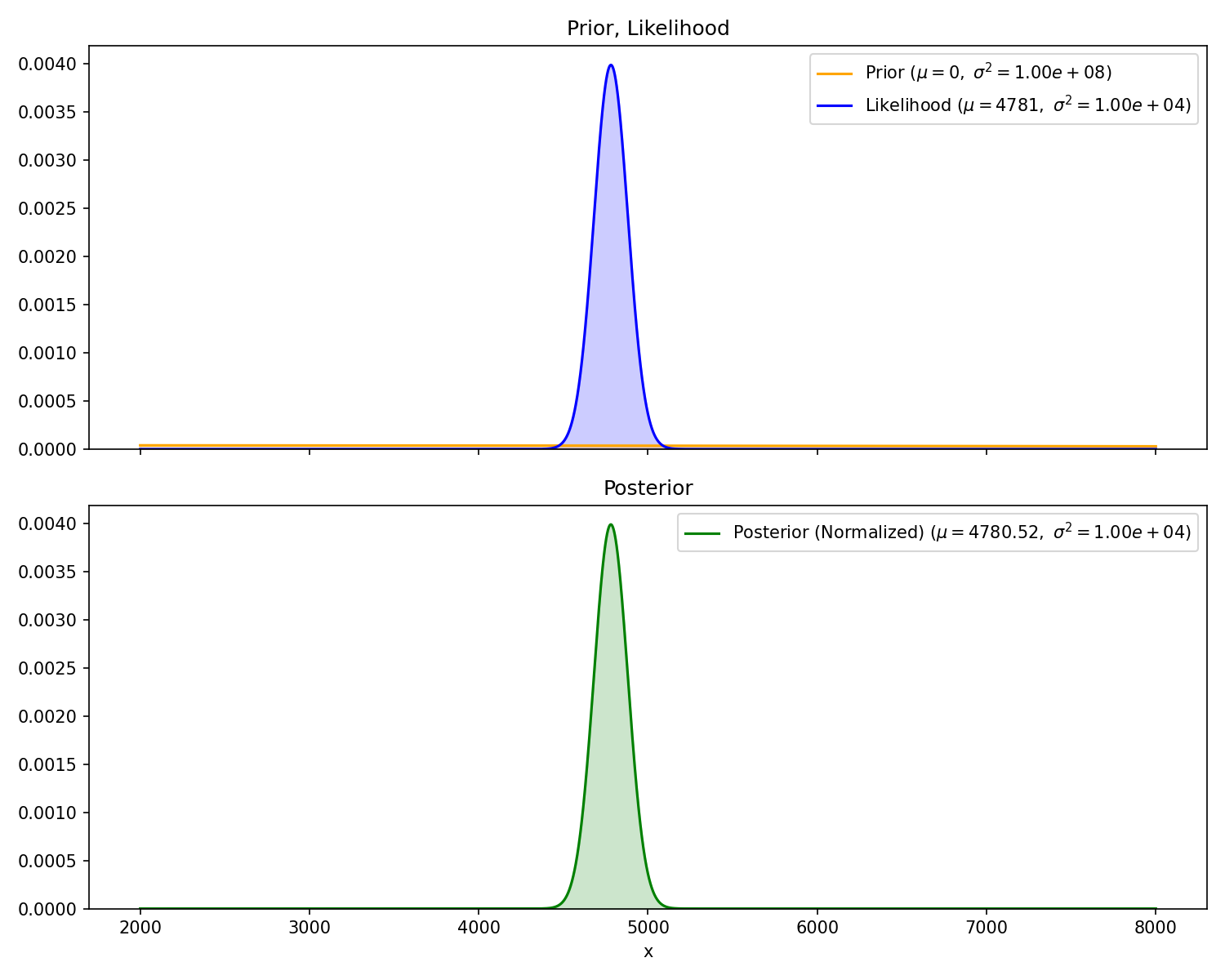
We need two things to calculate our posterior. First, the prior f_X(x). This represents our belief about the other sub’s position before receiving any measurement. Since we don’t have any a-priori knowledge, we can use a Gaussian distribution with extremely high variance (i.e., very flat) which loosely says “it could be anywhere”.
f_X(x)=\mathcal{N}(\mu=0, \sigma^2=10^8)=\frac{1}{\sqrt{10^8\times2\pi}}\exp\left(-\frac{1}{2}\left(\frac{x^2}{10^8}\right)\right)
Aside: however wide, this prior is not uniform: it has slightly more probability around 0 than at 1000m. We can’t make our prior’s variance infinite as that is ill defined, but we could have used an uninformative, improper prior. “Uninformative” meaning it contains no information (uniform everywhere) and “improper” because it doesn’t integrate to 1. While I won’t go into more detail here, I point it out because sometimes people say you can “initialize the particle filter using the first measurement” (i.e., use the normalized likelihood function of the first measurement as your prior), but really what they’re doing is applying Bayes’ rule with an uninformative prior.
Second, we need our likelihood function, f_{Y|X=x}(y). This is defined as the probability of measuring y given the state, x. The problem statement directly gives this to us: “The sonar readings are centered on the true distance with standard deviation of 100”. Here, the “true distance” is x
f_{Y|X=x}(y)=\mathcal{N}(\mu=x, \sigma^2=10^4)=\frac{1}{\sqrt{10^4\times2\pi}}\exp\left(-\frac{1}{2}\frac{(y-x)^2}{10^4}\right)
Now, we can plug these into Bayes’ theorem and solve for the posterior f_{X|Y=y}(x). Fortunately, the product of two Gaussian Distributions is also Gaussian (proof) with mean and variance
\sigma=\sqrt{\frac{\sigma_1^2\sigma_2^2}{\sigma_1^2+\sigma_2^2}},\quad\mu=\frac{\mu_1\sigma_2^2+\mu_2\sigma_1^2}{\sigma_1^2+\sigma_2^2}
The denominator (evidence), f_Y(y), is a scalar value (remember, y is given). Therefore, the posterior is also a Gaussian. I won’t go through the entire derivation here, but understand the solution is analytical
Aside: an analytical solution is derived by moving around variables with pencil and paper (e.g., anything you did in a high school algebra class). It is exact. Numerical solutions, on the other hand, are calculated via an algorithm and are approximate. They typically incur some discretization or rounding error which approaches zero in the limit of infinite memory or compute time.
I’ll note a few things. First, the prior is hard to see because it is pretty close to a flat line right around 0. Second, the mean of the posterior is very slightly less than the measurement. This is because our prior is centered at zero, so it will still “pull” the posterior towards it, no matter how flat it is. Third, the equation for the standard deviation, \sigma, above guarantees that the variance of the posterior is less than or equal to the variance of prior and likelihood Gaussians.
Now, we get a second measurement,
   🛥️ ···))·····))     🛥️
<───┼───────────────────┼───> x
0 ❓| Measurement | Range |
|---|---|
| #2 | 4952 meters |
And we’d like to update our probability distribution of the other submarine’s position, f_X(x). Recalling the math recap from the beginning, we can use the posterior from Act 1 as our new prior, rinse and repeat.
\text{Act 2 posterior} = \frac{\substack{{\text{measurement \#2}}\\ {\text{likelihood}}} \times \text{Act 1 posterior}}{\substack{\text{probability of measurement \#2 }\\{\text{across all possible x}}}}
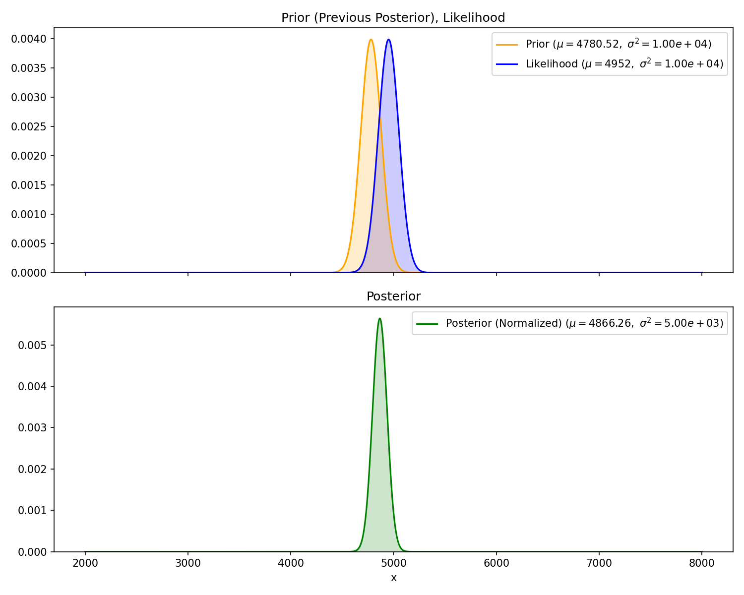
Again, the variance of the posterior is smaller than the two inputs. Since the variance of the prior and likelihood are roughly the same, the mean of the posterior is half way in between the two.
One of the powers of Bayesian inference is that it allows subjective priors. By that, I mean your domain knowledge and lived experience may give you a hunch that the other sub likes to hang out in some area and is therefore probably some distance away. Bayesian inference allows you to turn this “hunch” into a prior. This is possible because (in theory) no matter what prior you choose (so long as it is not zero where it matters) with enough measurement updates eventually your posterior will converge on the true distribution. Therefore we can leverage subjective “hunches” while maintaining some mathematical guarantees.
Now, the other submarine is moving, but we don’t know how fast. We take sequential sensor measurements. Our goal is to estimate (at the time of the last measurement) the velocity and range of the other submarine. We’ll make the following assumptions
   🛥️ ···))······))    🛥️💨
<───┼───────────────────┼───> x
0 ❓The state of the other submarine is now a random vector X:
x= \begin{bmatrix} x_1 \\ x_2 \end{bmatrix}= \begin{bmatrix} \text{position} \\ \text{velocity} \end{bmatrix}
And its probability distribution is now multivariate Gaussian X\sim\mathcal{N}(\mu,\Sigma). Our prior is
\mu =\begin{bmatrix} 0 \\ 0 \end{bmatrix}, \quad \Sigma=\begin{bmatrix} 10^8 & 0 \\ 0 & 5 \end{bmatrix}
Again, we will employ Bayesian inference. The problem is now two dimensions, but conceptually the technique is the same. We will treat the first measurement just as we did in Act 2. However, after calculating the posterior f_X(x) of the random vector, instead of immediately turning it into our next prior, we first must update it with time. To do this, we need something called a “motion model” or “state update equation”. Given a state at t-1, and our assumption of constant velocity, the state at t is given by
\textrm{pos}_t=\textrm{pos}_{t-1}+\text{vel}_{t-1}\Delta t \\ \textrm{vel}_t=\textrm{vel}_{t-1}
where \Delta t is the time in between each sensor reading. This is a linear transformation we can write in matrix form:
\begin{bmatrix} \text{pos} \\ \text{vel} \end{bmatrix}_t = \begin{bmatrix} 1 & \Delta t \\ 0 & 1 \end{bmatrix} \begin{bmatrix} \text{pos} \\ \text{vel} \end{bmatrix}_{t-1} = A \begin{bmatrix} \text{pos} \\ \text{vel} \end{bmatrix}_{t-1}
(I’m sticking with convention here to call this matrix A).
Given a state vector we can transform it with time, but how do we transform a continuous distribution? Let’s change our framing slightly; instead of thinking about probability distributions, let’s consider the random variable X=\{\text{pos},\text{vel}\} which this distribution describes. Again, we are fortunate that our variable is Gaussian. Thinking back to an intro stats class, you may remember that multiplying a random variable by a constant b scales its mean by b and its variance by b^2. This extends to random vectors. Given any linear transformation Y=BX,
E[Y]=B E[X]
Cov(Y)=B Cov(X)B^T
Because the Gaussian distribution is defined by this mean and variance, the resulting distribution of our random variable is also Gaussian with
\mathcal{N}(\mu,\Sigma)\to \mathcal{N}(A\mu,A\Sigma A^T)
So long as our motion model is a linear transformation and our prior and measurements are still Gaussian, the posterior will remain Gaussian, and therefore the entire process can be solved analytically. Say we receive the following three measurements:
| Measurement | Time | Range |
|---|---|---|
| #1 | 0 seconds | 7507 meters |
| #2 | 60 seconds | 7671 meters |
| #3 | 200 seconds | 8099 meters |
To process the first, we apply Bayes’ theorem just as we did in Act 2. I’ve plotted top-down heatmaps of our probability distributions. Getting oriented, an informationless prior would look like a uniform, light orange background. Our prior is a bit better than informationless: we know the velocity is probably between \pm 4 m/s.
Our sensor still provides only range information. Therefore it appears as a 1D Gaussian smeared uniformly across the velocity axis.
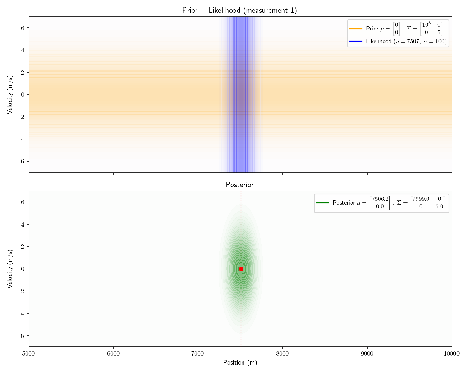
Aside: I haven’t plotted the actual prior here – it would appear as a single color. I’ve emphasized things for visual effect.
Notice how the posterior mean is slightly lower than 7507. This is because our prior is not truly “informationless” it is just a very flat Gaussian centered at 0, so it will pull the posterior slightly towards 0.
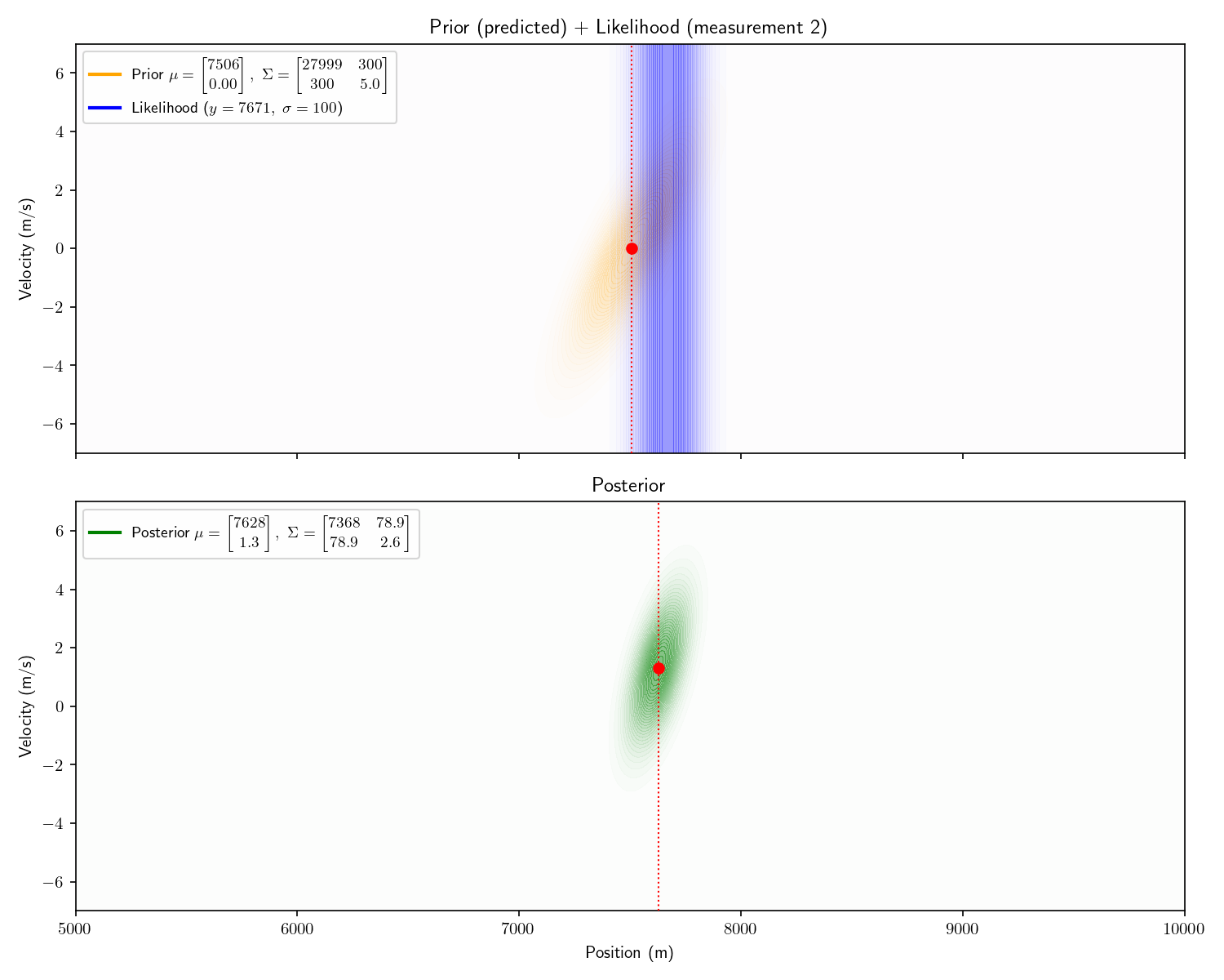
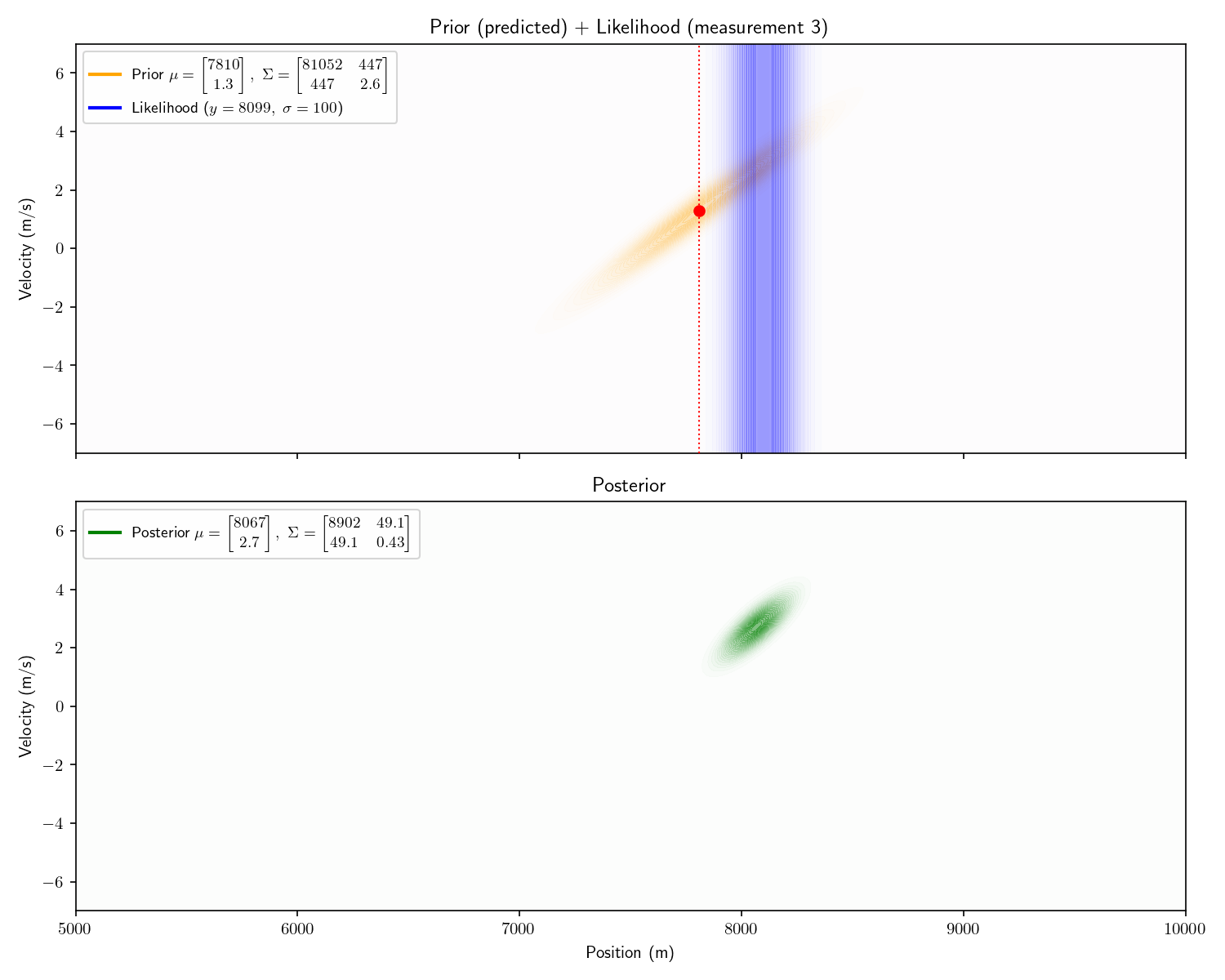
Aside: the first posterior’s covariance matrix has 0s in its off diagonals. This is a fancy way of pointing out that it isn’t slanted. After we apply the motion model, these off-diagonal elements become non-zero and it becomes slanted. It is this covariance matrix that carries the “information” about the relationship between the possible positions and velocities: i.e., “If the sub has a positive velocity it is probably further away now”.
Let’s zoom out for one moment. Our goal is to motivate the particle filter. Until this point we haven’t defined “particle” or “filter”. The approach I’ve just described is is called “recursive Bayesian estimation” or a “Bayesian Filter”. The first phrase describes exactly what we’ve done: recursively apply Bayes’ theorem to estimate the state of the submarine. As for the latter, “filtering” simply means we are estimating the state of the submarine at the time of the last measurement as opposed to during the whole encounter. At this point you know literally 1/2 of “particle filter”, and our conceptual understanding is roughly half way there as well.
In particular, a Bayesian filter where the prior and measurements are Gaussian and the state update is linear is called a “Kalman Filter”.
Notice one more thing about our results. Our final posterior tells us that the other submarine’s velocity is between +2 and +4. This is remarkable because we never received any information about its velocity! We call velocity a “hidden state” because it is never observed. One powerful trait of Kalman Filters is that they can provide estimates of states which are never observed.
Aside: the Kalman filter can also represent Gaussian noise in the state update. For example, imagine the velocity of the submarine depended on the temperature/salinity of the water. We could model the effect of this unknown environment as Gaussian noise (just like we did with the measurements).
Aside: the “extended Kalman filter” (EKF) can use any differentiable function for the state-transition model (rather than linear). This involves constructing a Jacobian (matrix of partial derivatives) to update the covariance with. The EKF is the de facto technique of GPS systems.
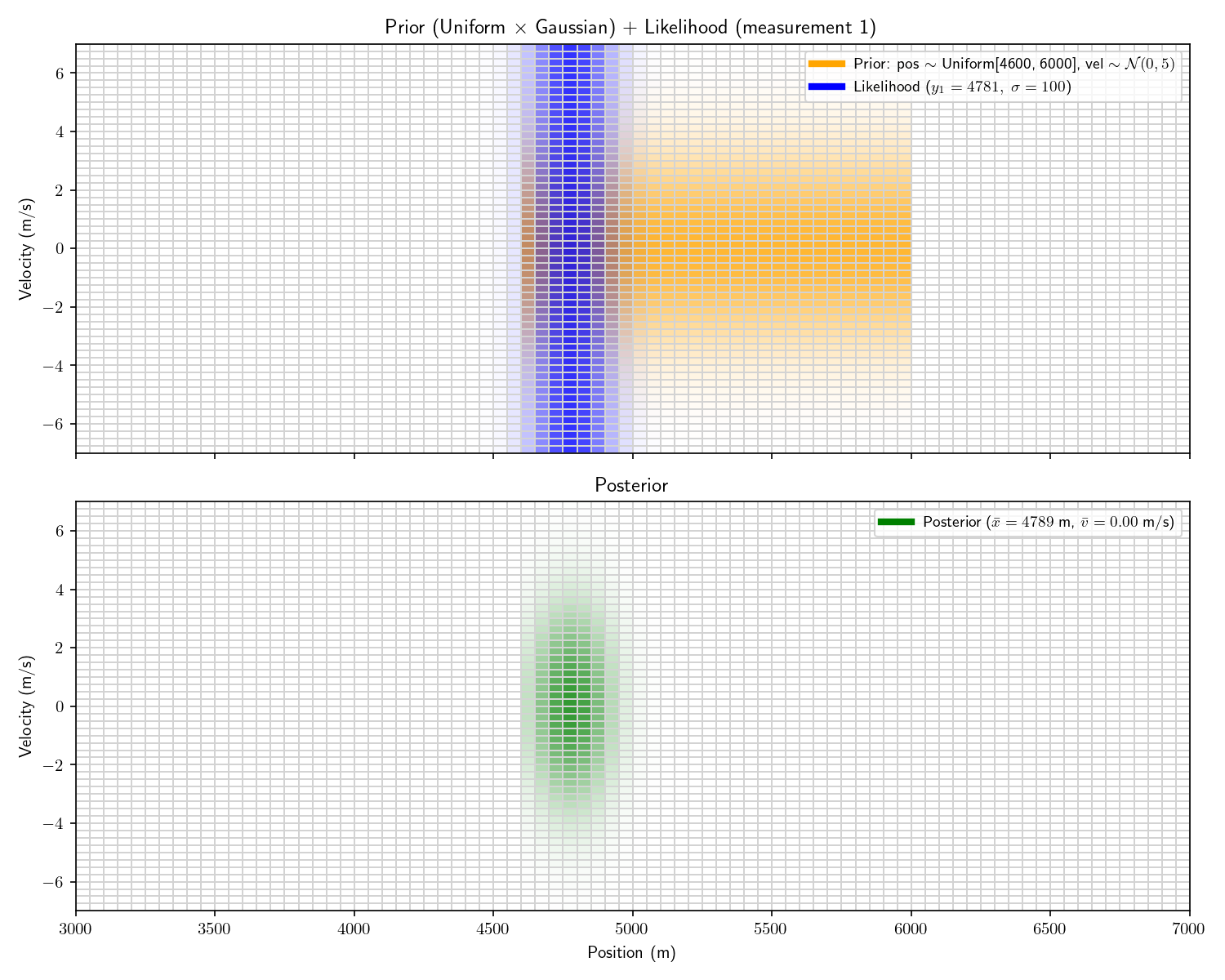
Now imagine that before receiving the first sensor report, we receive an intelligence that the other submarine is between 4,600 and 6,000 meters away.
   🛥️ ···))······))       🛥️
<───┼────────────────┼──────────┼───> x
0                  4,600  ❓  6,000
And then we receive the following three measurements:
| Measurement | Time | Range |
|---|---|---|
| #1 | 0 seconds | 4781 meters |
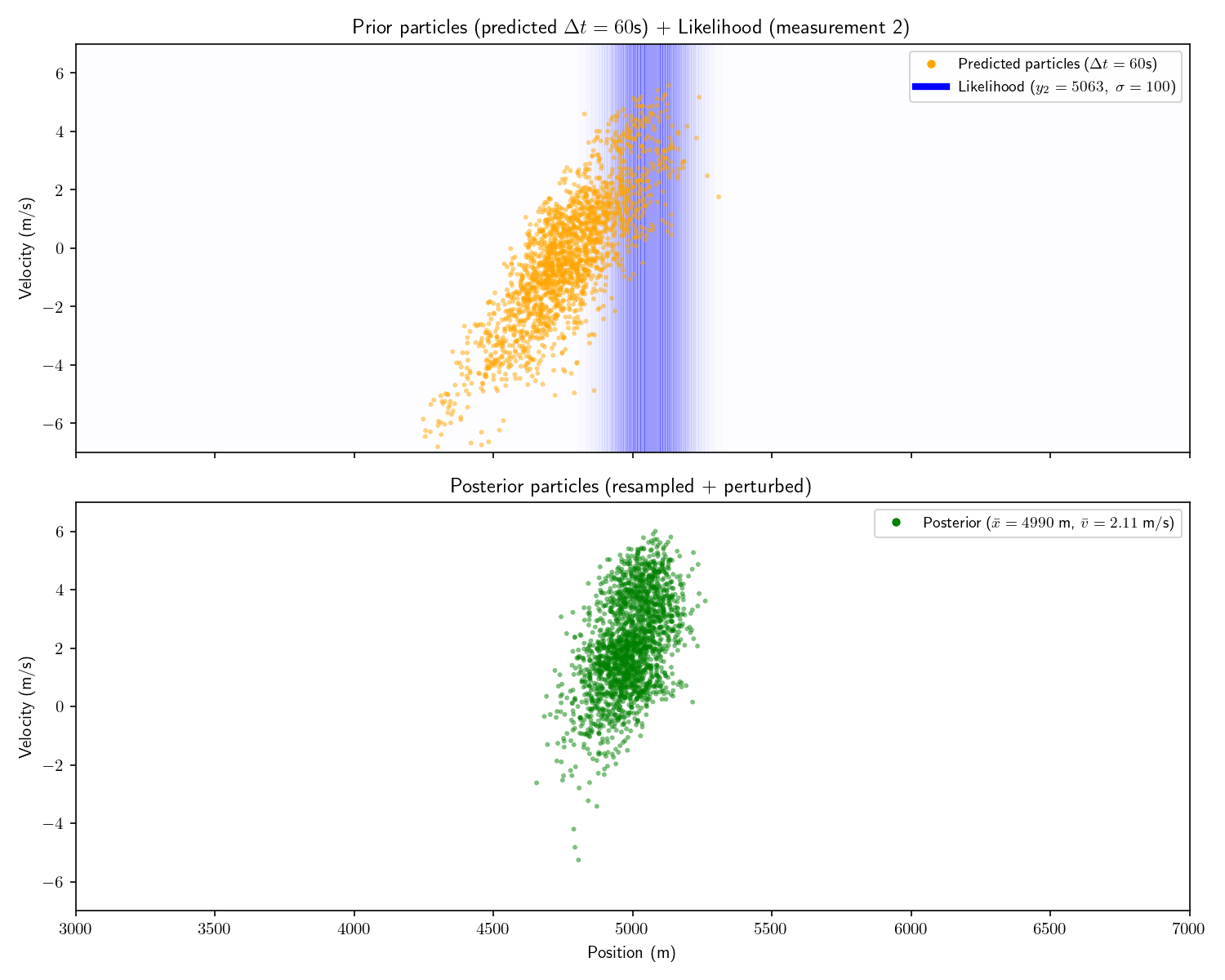
| #2 | 60 seconds | 5063 meters |
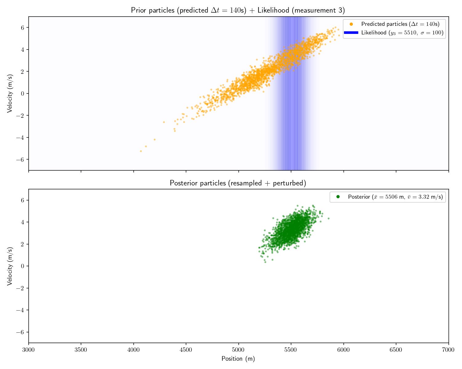
| #3 | 200 seconds | 5510 meters |
We can incorporate the intelligence report into our Bayesian framework as a uniform prior:
f_X(x) = \frac{1}{\text{1,400}} \quad \text{for } x \in [\text{4,600}, \text{6,000}]
The problem with a uniform prior is that we can no longer solve the problem analytically. What can we do instead? One option divide the x-dimension into 200 “bins” then calculate the prior and likelihood for each bin. Then, using the same linear motion update
\begin{bmatrix} \text{pos} \\ \text{vel} \end{bmatrix}_t = \begin{bmatrix} 1 & \Delta t \\ 0 & 1 \end{bmatrix} \begin{bmatrix} \text{pos} \\ \text{vel} \end{bmatrix}_{t-1} = A \begin{bmatrix} \text{pos} \\ \text{vel} \end{bmatrix}_{t-1}
For each bin in step (t-1)’s posterior, transform its state x_1 into x_2 using A and add that probability to step t’s prior’s bin at x_2.
Aside: alternatively we could have used a Gaussian prior with (\mu=5,300, \sigma=700), called it close enough, and used a Kalman Filter. This sounds hacky, but it’s often often a good option.
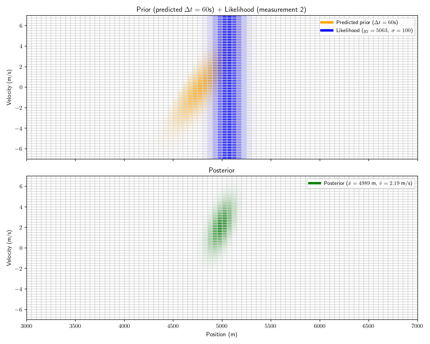
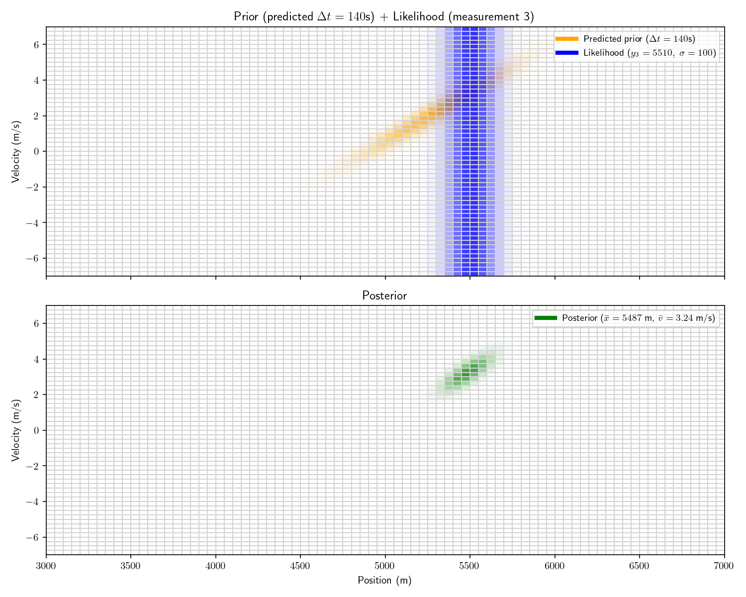
Let’s take one more step back. What we’ve just constructed is called a “Histogram Filter”. Our solution is no longer analytical – that is we’ve approximated our continuous distributions with a finite grid. This sacrifices some precision, but allows us to consider non-Gaussian priors.
In this Act we used the same motion model A as in Act 3. However, now that we’ve abandoned the requirement of an analytical solution, our motion model no longer needs to be linear either. So long as we can come up with a way to “update” the probability in the posterior forward in time, we can do so however we wish. For example, say we know that every 10 minutes the other submarine turns around. We could have a literal if-else statement in our motion update that if t\%(10*60)==0, negate the velocity. This is impossible with a Kalman Filter.
Finally, note that while our measurements have remained Gaussian they need not have. Once we start solving things numerically, we can drop any requirements about functions being Gaussian.
Now let’s consider a higher-dimensional problem: both submarines move in three dimensions. We would like to track both position \{x,y,z\} and velocity \{v_x,v_y,v_z\}. Assume our measurements are 3d Gaussians on \{x,y,z\} and our prior is a uniform distribution over a cube in \{x,y,z\}.
If, like before, we split each dimension into 200 bins, we now have 200^6=64\;\text{Trillion} bins. Using one float (32 bits) to store each bin’s value would require 32\times 64\times 10^{12} \;\text{bits}\approx250\;\text{Terabytes}. This is an example of “the curse of dimensionality”.
Let’s think about what’s happening here. In our 2-dimensional example, after 3 measurements we are almost certain the other submarine has a positive velocity. We nonetheless multiply the prior (0) by the likelihood (0) to get the posterior (0) for every bin with negative velocity. This is a tremendous waste of compute. There are some tricks like having a dynamic discretization: have very wide bins where there is no probability and very small grids where the probability is non-zero. Possible, but adds quite a bit of complexity.
Note that the Kalman filter does not suffer from the curse of dimensionality. Since it only needs to keep track of the mean and covariance matrix, which, in 6 dimensions only require 42 floats.
Aside: the idea of assuming a Gaussian distribution to avoid the curse of dimensionality is not unique to the Kalman Filter. In machine learning, Quadratic Discriminant Analysis and Naive Bayes leverage this idea.
The particle filter solves this problem. Instead of moving our probability between bins, leaving many bins with zero probability, why not move the bins themselves? Call these moving bins “particles”. Each particle is comprised of its state \{\text{position},\text{velocity}\} and its probability which we call its “weight”.
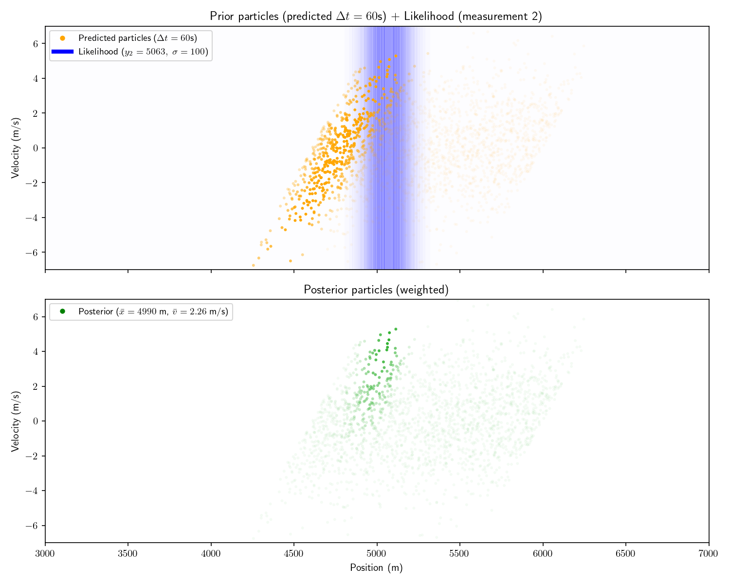
To construct our set of particles, sample from the first prior distribution. There is no longer a need to discretize our likelihood functions as we can evaluate them directly at the state of each particle. After applying the likelihood function, we update each particle using our state-transition model A. Like the histogram filter, we need not use a linear state-transition model or Gaussian prior/likelihoods. Note that the superscripts denote the particle index, not an exponent. Typically, the subscript is reserved for the time index.
\text{particle 1 (state}\ x^1):\quad x^1_t = \begin{bmatrix} 1 & \Delta t \\ 0 & 1 \end{bmatrix} x^1_{t-1}
\text{particle 2 (state}\ x^2):\quad x^2_t = \begin{bmatrix} 1 & \Delta t \\ 0 & 1 \end{bmatrix} x^2_{t-1}
\vdots
At each step the prior is the set of original particles and their weights and the posterior is the set of particles with updated weights. Each particle’s weight is updated according to Bayes’ theorem.
\text{particle 1 (state}\ x^1):\quad \text{new weight} \propto \frac{\substack{{\text{likelihood of sensor }}\\ {\text{reading y given }x^1}} \times \text{old weight}} {\text{evidence}} \propto \text{likelihood}\times\text{old weight}
\text{particle 2 (state}\ x^2):\quad \text{new weight} \propto \frac{\substack{{\text{likelihood of sensor }}\\ {\text{reading y given }x^2}} \times \text{old weight}} {\text{evidence}} \propto \text{likelihood}\times\text{old weight}
\vdots
I’ve written “\propto” (proportional to) instead of “=” because there is one more step to calculate the new weight. The particles comprise a probability distribution, so the sum of their weights should sum to 1. Therefore, we divide each weight by their sum. The effect of this normalization is the same regardless of any constant factor, so we can ignore the evidence constant.
Aside: people often get lazy and say “the particle’s likelihood”. This is short for “the likelihood of the measurement conditioned on the particle’s state”. Particles don’t have likelihoods.
For consistency, I’ll show the same 2D example as from Act 5. It’s important to understand that this technique can scale to higher dimensions, but things are simpler to visualize in 2D.
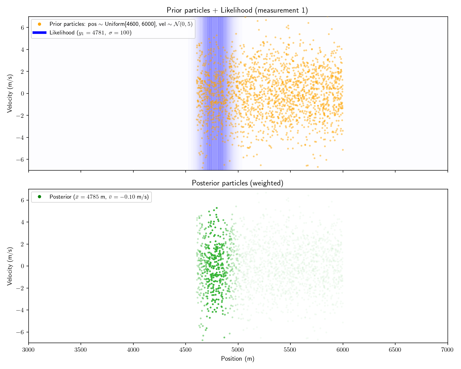
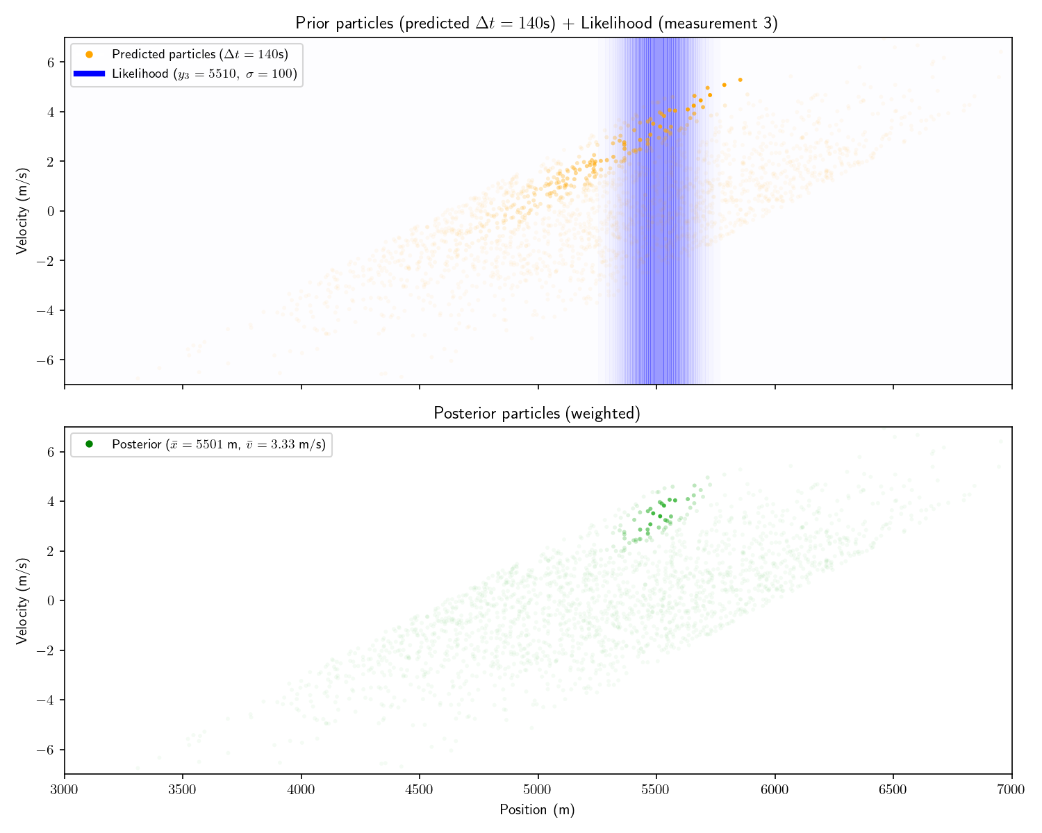
Note that in these plots I’ve set a floor on the opacity of each particle to help visualize things. Had I let the opacity go to zero, the very opaque particles would all disappear.
I’ll pause here and say that a particle filter with infinite particles and a histogram filter with infinite bins, will converge on the same analytical posterior provided by a Kalman filter. Of course, we’re doing all this to avoid trillions of cells let alone infinite ones, but it’s good to know things will converge to the correct answer. Everything from here on is a trick to use less compute, not a mathematical requirement.
Aside: what I’ve described here is called a “bootstrap filter”. It is a particular kind of particle filter where certain assumptions are made so that \text{new weight}\propto \text{likelihood}\times\text{old weight}. This isn’t always the case. I’ve omitted the mathematical details since I don’t think they are necessary for a conceptual understanding. You can read more on Wikepdia here.
My critique of the histogram filter was that it wasted effort computing bins which had zero probability. We could make the same critique here: most of the particles have near-zero weight but we keep them around.
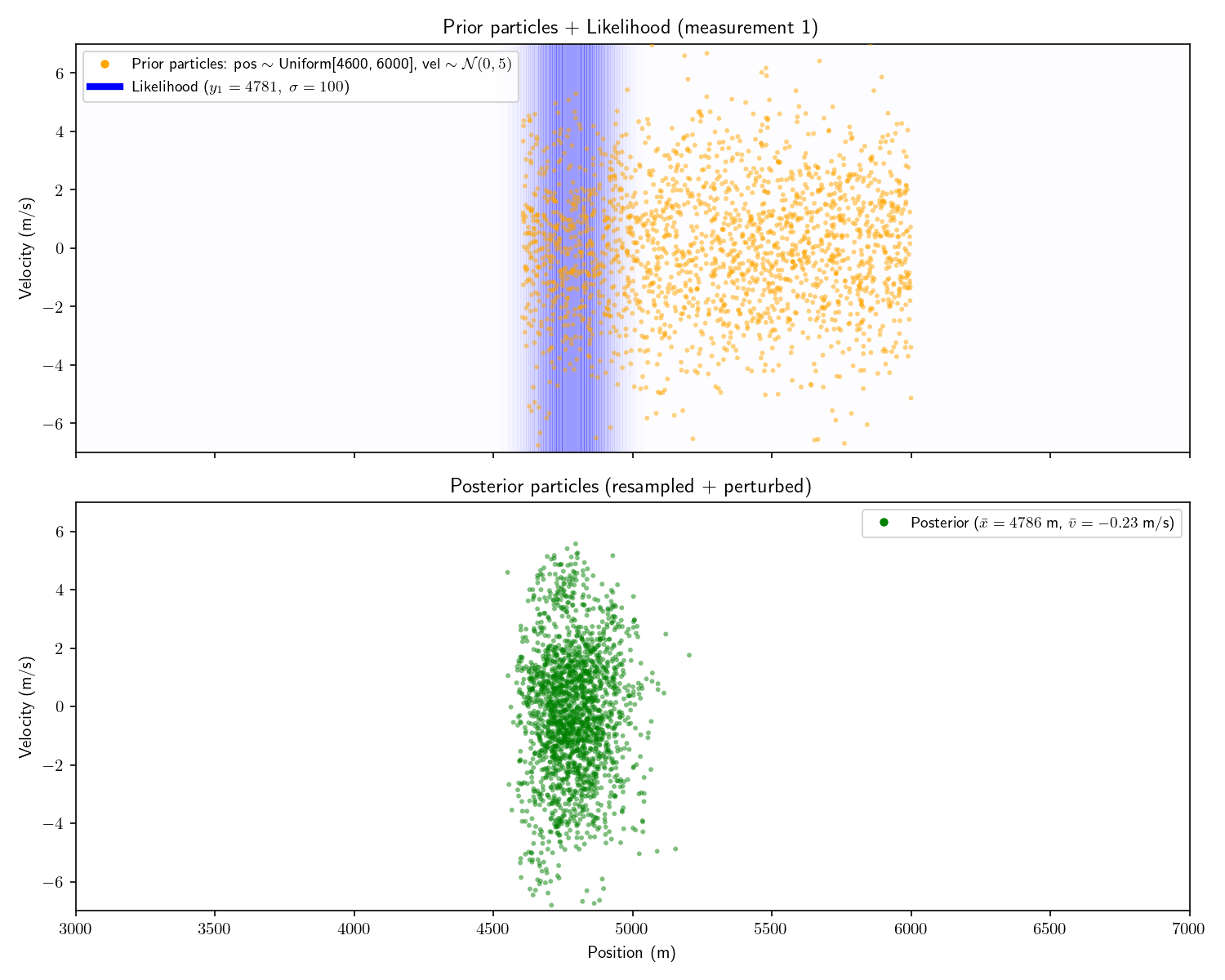
The solution is to “resample” the particles. Imagine we have 100 particles. Originally each has weight 1/100. After performing the measurement update, half have weight zero and half have weight 1/50. To resample we throw away the particles with 0 weight and duplicate each of the survivors. We’re left with a total weight of 1 and our surviving particles are all in the “region of interest”. I won’t go into more detail about resampling, there is no shortage of explainers on the internet which focus on it.
A common technique which accompanies resampling is to add “perturbations” to the resampled particles. That is, add a bit of Gaussian noise to each perturbed particle’s state. This is because we only have finite particles, so we would like to “smear out” the survivors to more evenly cover the space.
Aside: it’s at this point that things start becoming more of an art than a science. As you progress developing a particle filter, more and more decisions will start to fall in the former category
Here are the results of adding resampling and perturbing to our particle filter:
Fair warning: particle filters fall apart in high dimensions. There just aren’t enough particles to cover the space (curse of dimensionality). Things fare better if things are roughly Gaussian.