7/13/25
This post extends my midterm project for Plasma Physics 615.753 at Johns Hopkins. The project was open-ended: explore a particle motion you’re interested in. I’m sharing because I’m happy with my results and hope someone learning the material finds them useful. In particular, there aren’t many guides to the poloidal/toroidal coordinate system or casual introductions to particle drifts in tokamaks. (Python code)
If held in a plasma of high enough temperature and density, light ions will eventually fuse. Magnetic confinement is an approach to controlled fusion which achieves these conditions using the magnetic force. This force acts perpendicular to ions’ velocity and the magnetic field, causing them to travel in helices around field lines. Tokamaks bend these field lines into a torus, trapping ions like beads on a bracelet. Once this trap is set, ions are injected and heated with electromagnetic radiation to achieve fusion conditions. Unfortunately, the centers of ion orbits drift away from their original field lines causing them to escape confinement. The addition of a poloidal (short way around the torus) component to the magnetic field negates the effect of this drift. This post derives a representative magnetic field using a toroidal/poloidal coordinate system and motivates the additional poloidal component by simulating the trajectory of a single particle.
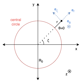
It’s much simpler to formulate a tokamak’s magnetic field using a toroidal/poloidal coordinate system because its geometry mirrors the problem’s, encapsulating its complexity. This system describes locations relative to a “central circle” of radius R_0 using three coordinates: r, \theta, and \zeta. \zeta measures the toroidal angle (long way around), \theta the poloidal, and r the distance from the central circle.
The translation to and from Cartesian coordinates is given by \begin{aligned} &x = (R_0+r\cos\theta)\cos\zeta\quad&r = \sqrt{(\sqrt{x^2+y^2}-R_0)^2+z^2}\\ &y = (R_0+r\cos\theta)\sin\zeta\quad&\theta = \arctan2(z, \sqrt{x^2+y^2}-R_0)\\ &z = r\sin\theta\quad&\zeta = \arctan2(y, x)\\ \end{aligned}
Where \arctan2(y, x) is the C/Python function which returns the angle between the positive x-axis and the point (x, y) in the plane. Notice that \sqrt{x^2+y^2}-R_0 is the signed distance to the central circle in the xy-plane where a negative value indicates the point is within the circle.
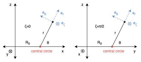
The unit vectors in this system (blue vectors in the figures), expressed in Cartesian coordinates, are \hat{r}= \left( \begin{array}{c} \cos\theta \cos \zeta \\ \cos \theta \sin \zeta \\ \sin \theta \\ \end{array} \right),\; \hat{\theta}= \left( \begin{array}{c} -\sin\theta\cos\zeta \\ -\sin\theta\sin\zeta \\ \cos\theta \\ \end{array} \right),\; \hat{\zeta}= \left( \begin{array}{c} -\sin\zeta \\ \cos\zeta \\ 0 \\ \end{array} \right)
Therefore, to translate a field vector with base (r, \theta, \zeta) and components (a, b, c) to Cartesian coordinates, the base can be found using the translation above, and the vector using the scaled unit vectors: \begin{aligned} \mathbf{p}&=a\hat{r}+b\hat{\theta}+c\hat{\zeta}\\ \mathbf{p}&=(a\cos\theta\cos\zeta-b\sin\theta\cos\zeta-c\sin\zeta)\hat{x}\\ &+(a\cos\theta\sin\zeta-b\sin\theta\sin\zeta+c\cos\zeta)\hat{y}\\ &+(a\sin\theta+b\cos\theta)\hat{z} \end{aligned}
If you pay close attention to the figures above, you’ll notice that the coordinate system is left-handed. That is, you can point your left thumb in \mathbf{e}_r, left index in \mathbf{e}_\theta and your middle will naturally point in \mathbf{e}_\zeta. This means that the cross product between vectors in order (r, \theta, \zeta) does not act like it does between (x, y, z). If using equations defined for a right-handed system, you would need to account for this with appropriate negative signs. Alternatively, you can make this system right-handed by measuring \theta or \zeta in the opposite direction. Since I only use this system to define the magnetic field and not do any calculations, this isn’t a concern.
The simplest field to imagine is a torus with constant magnitude in the \hat{\zeta} (toroidal) direction. \begin{aligned} \textbf{B}(r, \theta, \zeta)=\begin{cases} 1\hat{\zeta} & \text{if } r < r_0 \\ 0 & \text{otherwise} \end{cases} \end{aligned}
Where r_0 is the poloidal radius. Remember that the major radius R_0 is implicit in the coordinate system. Unfortunately, such a field is impossible to construct. Consider the integral around the central circle. Since the field is constant, the integral will be proportional to the loop’s radius. The integral over a loop with a slightly larger radius will be slightly larger. This contradicts Ampere’s law which tells us the integrals must be equal because the same amount of current (from the toroidal field coils) passes through each loop. In order to obey Ampere’s law, the magnitude of the magnetic field must vary with 1/R:
\begin{aligned} &\oint_{C_t} \textbf{B}_t\cdot d\ell=\mu_0I_{\textrm{enc}}\quad\textrm{(Ampere's law, $C_t$ is a toroidal loop)}\\ &\oint_{C_t} B_t d\ell=\mu_0I_{\textrm{enc}}\quad\textrm{(B is purely toroidal, parallel to }C_t)\\ &B_t\oint_{C_t} d\ell=\mu_0I_{\textrm{enc}}\quad\textrm{(B has toroidal symmetry)}\\ &B_t\int_0^{2\pi} R d\theta=\mu_0I_{\textrm{enc}}\quad\textrm{(R is the radius of }C_t)\\ &B_tR = \frac{\mu_0I_{\textrm{enc}}}{2\pi}=\textrm{Constant}\Rightarrow B_t\propto\frac{1}{R} \end{aligned}
Accounting for this fact leads us to the field: \begin{aligned} \textbf{B}(r, \theta, \zeta)=\begin{cases} R_0/(R_0 + r\cos\theta)\hat{\zeta} & \text{if } r < r_0 \\ 0 & \text{otherwise} \end{cases} \end{aligned} Since R=R_0+r\cos\theta. Choosing a numerator of R_0 normalizes this so that the field along the central circle 1.
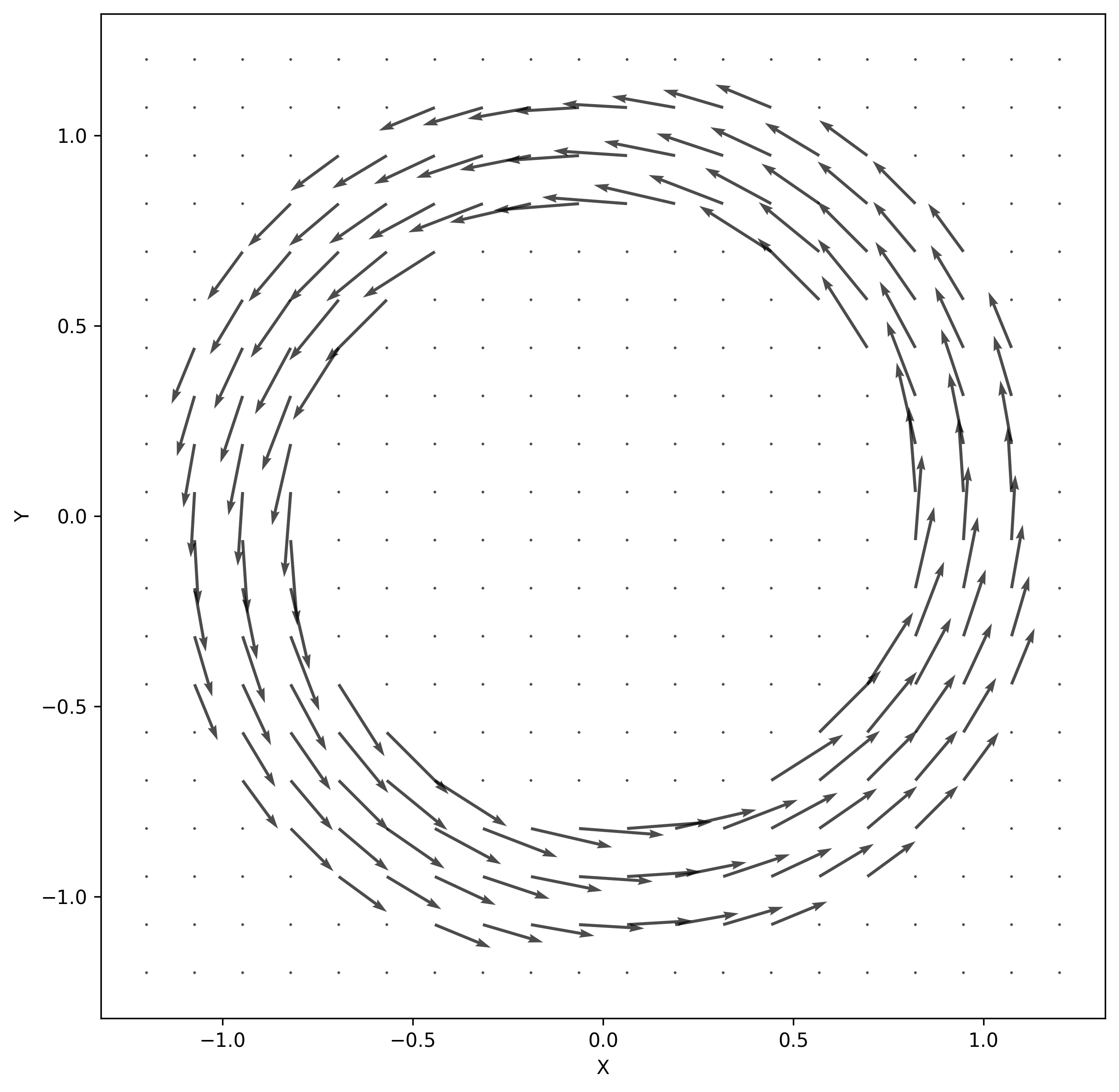
Look closely, and you’ll see that the length of the vectors on the inner radius are longer than those on the outer radius.
The addition of a poloidal field helps mitigate particle drift (I’ll explain why in the next section). It’s not possible to create such a magnetic field with external coils, so instead, Tokamaks drive a toroidal current through the plasma itself. The precise mechanism (induction, neutral beam injection, or electromagnetic radiation) is not important here. Assuming this current density \textbf{J} is uniform:
\begin{aligned} &\oint_{C_p} \textbf{B}_p\cdot d\ell=\mu_0I_{\textrm{enc}}\propto J\pi r^2\quad\textrm{(Ampere's Law, $C_p$ is a poloidal loop)}\\ &\oint_{C_p} B_p d\ell\propto r^2\quad(B_p\textrm{ is purely poloidal, parallel to }C_p)\\ &B_p\oint_{C_p} d\ell\propto r^2\quad(B_p\textrm{ has poloidal symmetry)}\\ &B_pr \propto r^2\Rightarrow B_p\propto r \end{aligned}
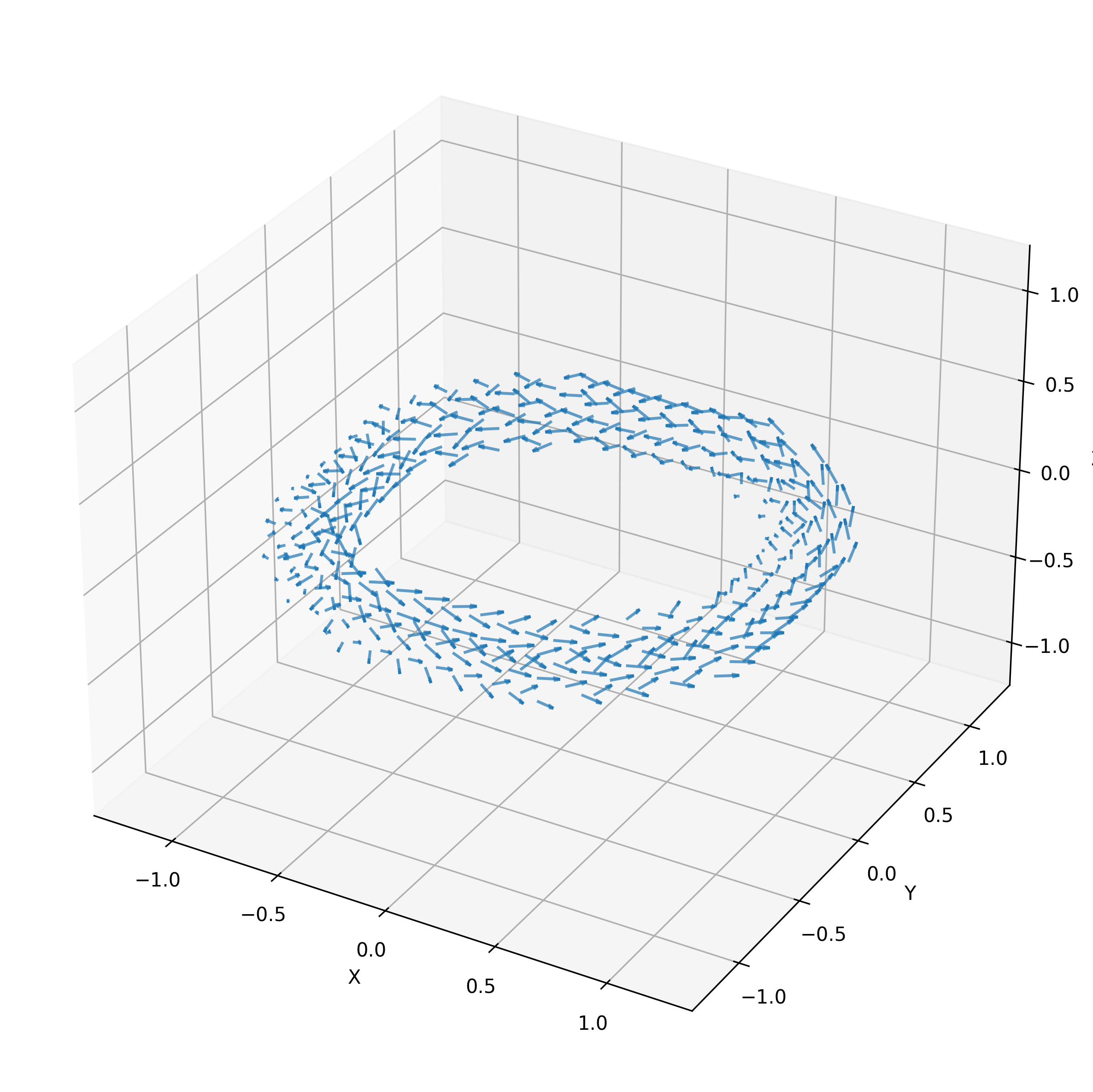
Ampere’s law tells us that this poloidal field is proportional to the minor-distance from the central circle, r. Because the magnetic field in a vacuum linear, the toroidal \textbf{B}_t and poloidal fields \textbf{B}_p can be combined by addition:
\begin{aligned} \textbf{B}(r, \theta, \zeta)=\begin{cases} R_0/(R_0 + r\cos\theta)\hat{\zeta} + (r/r_0) \hat{\theta} & \text{if } r < r_0 \\ 0 & \text{otherwise} \end{cases} \end{aligned}
I normalize the poloidal \hat{\theta} term, so it varies from 0 at the central circle to 1 at the surface.
There are two causes of particle drift due to complexities of the magnetic field. The first is caused by the magnetic field varying in magnitude. This is called grad-B (\nabla B) drift. It causes the orbital centers of particles to move with velocity:
\mathbf{v}_{\nabla B}=\pm\frac{1}{2}v_\perp r_L\frac{\mathbf{B}\times\nabla B}{B^2},\quad r_L=\frac{mv_\perp}{|q|B} Where v_\perp is the particle’s velocity perpendicular to the field line, r_L is the Larmour radius (radius of a single orbit around the field line), and B=|\textbf{B}| is the magnitude of the magnetic field. The \pm indicates that the drift is positive for ions and negative for electrons. To calculate this drift for the toroidal field, consider an ion anywhere in the poloidal cross-section at \zeta=0. Using the fact that when \zeta=0, \hat{\zeta}=\hat{y} and that x=R_0+r\cos\theta, we can write the gradient of the field in Cartesian coordinates.
\begin{aligned} &\textbf{B}=R_0/(R_0+r\cos\theta)\hat{\zeta}=(R_0/x) \hat{y}\\ &B=R_0/x\\ &\nabla B=\frac{\partial B}{\partial x}\hat{x}=-\frac{R_0}{x^2}\hat{x} \end{aligned}
The grad-B drift for an ion with charge q and mass m is then
\mathbf{v}_{\nabla B}=\frac{1}{2}v_\perp\frac{mv_\perp}{q(R_0/x)}\frac{(R_0/x)\hat{y}\times(-R_0/x^2)\hat{x}}{(R_0/x)^2}=\frac{mv_\perp^2}{2qR_0}\hat{z}
By argument of symmetry (we could have oriented the x-axis however we like) the ion will experience this same drift everywhere in the torus. Notice this is a constant, so this drift is the same for any particle trajectory.
The second type of drift is due to the curvature of the field and arises from the centrifugal force: \textbf{v}_R=\frac{mv_\parallel^2}{qB^2}\frac{\textbf{R}_c\times\textbf{B}}{R_c^2} Where \textbf{R}_c is the vector pointing from the center of the torus to the particle, and v_\parallel is its velocity along the magnetic field line. Now consider an ion at \zeta=\theta=0, that is, along the x-axis so that R_c=x. The curvature drift will be \textbf{v}_R=\frac{mv_\parallel^2}{q(R_0/x)^2}\frac{R_c\hat{x}\times(R_0/x)\hat{y}}{R_c^2}=\frac{mv_\parallel^2}{qR_0}\hat{z}
If the particle has a non-zero z-component, this becomes more complex since R_c\neq x and \textbf{R}_c is no longer perpendicular to \textbf{B}.
The net effect in the toroidal field is that ions traveling in the direction of the field lines will drift in the +\hat{z} direction until they escape confinement. This is obviously a concern. Fortunately, the addition of a poloidal component of the magnetic field solves this problem. The twisting path causes ions to spend an equal amount of time in the top (z>0) and bottom (z<0) of the torus. While the ion is in the top, its upward drift causes it to move away from the central circle, but while it is in the bottom, its drift bring it back towards the central circle. Therefore, on average, there is no overall drift!
Assume the effect of gravity is negligible and the electric field is zero. The ion experiences only the magnetic force:
\begin{aligned} &\textbf{F}=m\textbf{a}=q\textbf{v}\times\textbf{B}\\ &\frac{d\textbf{v}}{dt}=\frac{q\textbf{v}\times\textbf{B}}{m}\\ \end{aligned}
The ion’s trajectory will follow this ODE. This cannot be solved analytically, so I use an adaptive Runge-Kutta method to solve it numerically. We can simplify the code by non-dimensionalizing this equation. That is, replace each component of the equation with a characteristic unit (denoted by a subscript c) multiplied by a non-dimensional term (denoted by ~). For example, a=\tilde{a}a_c
\begin{aligned} \left(\frac{v_c}{t_c}\right)\frac{d\tilde{\textbf{v}}}{d\tilde{t}}&=\left(\frac{q_cv_cB_c}{m_c}\right)\frac{\tilde{q}\tilde{\textbf{v}}\times\tilde{\textbf{B}}}{\tilde{m}}\\ \frac{d\tilde{\textbf{v}}}{d\tilde{t}}&=\left(\frac{q_cB_ct_c}{m_c}\right)\frac{\tilde{q}\tilde{\textbf{v}}\times\tilde{\textbf{B}}}{\tilde{m}}\\ \frac{d\tilde{\textbf{v}}}{d\tilde{t}}&=\frac{\tilde{q}\tilde{\textbf{v}}\times\tilde{\textbf{B}}}{\tilde{m}}\\ \end{aligned}
Fix q_c, B_c, and m_c to scales relevant to the problem, and then choose t_c so that this pre-factor becomes 1. Characteristic length is then derived from the other units.
The simulation will use this simplified, non-dimensional equation. To recover a dimensional-quantity, simply multiply the non-dimensional value by the characteristic unit.
I use the following parameters and initial conditions:
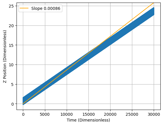
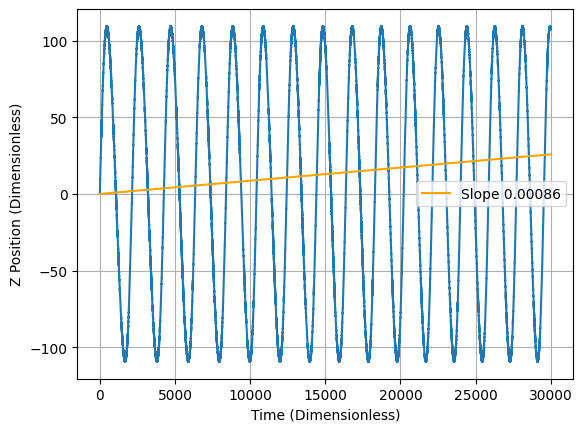
At the stating time, v_\parallel=v_y=v_\perp=v_x. Since v_\parallel^2+v_\perp^2=v^2, we have that v_\perp^2=v_\parallel^2=v^2/2, so the drift velocity should be roughly \begin{aligned} &\textbf{v}_{drift}=\textbf{v}_{\nabla B} + \textbf{v}_R=\left(\frac{mv_\perp^2}{2qR_0}+\frac{mv_\parallel^2}{qR_0}\right)\hat{z}\\ &\textbf{v}_{drift}=\left(\frac{mv^2}{4qR_0}+\frac{mv^2}{2qR_0}\right)\hat{z}=\left(\frac{3mv^2}{4qR_0}\right)\hat{z}\\ &\textbf{v}_{drift}=189\hat{z}\textrm{ m/s}=0.00086\hat{z} \end{aligned}
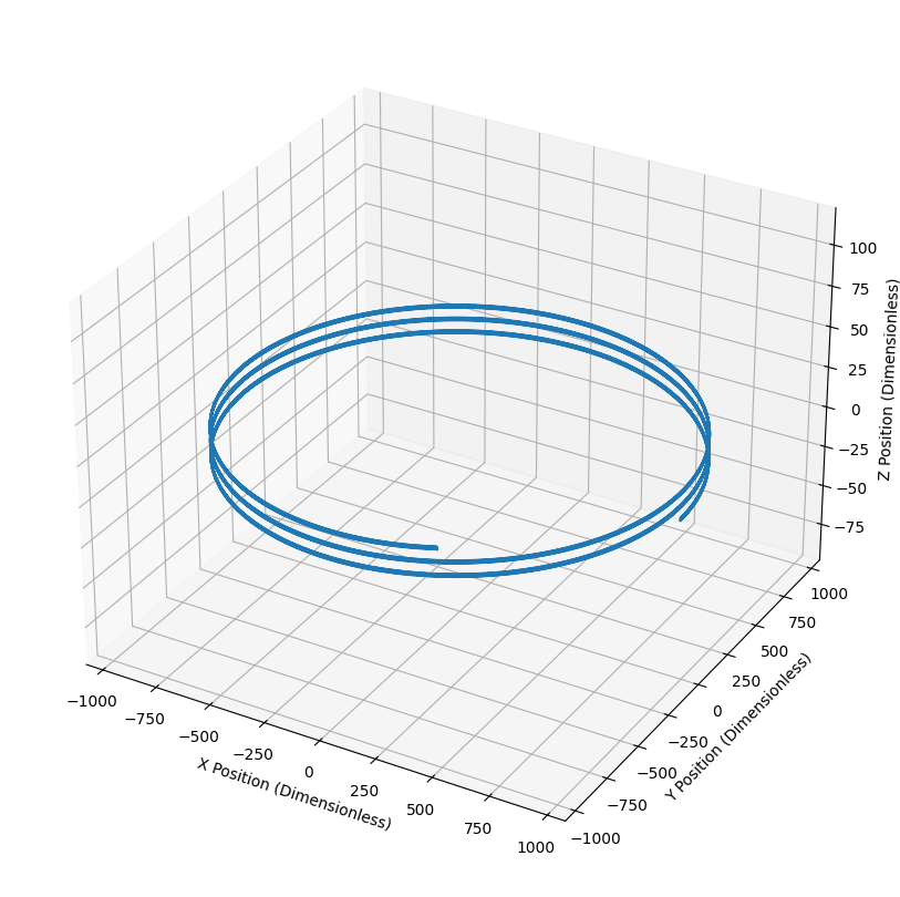
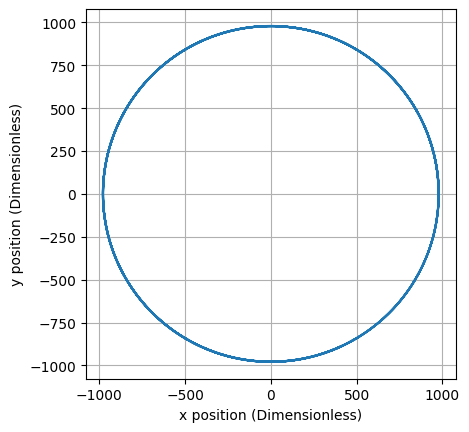
In the toroidal field, the particle follows a circular path while drifting upward as expected. The rate of this drift is slightly smaller than 0.00086. I don’t know why. Remember that while the particle loops the torus, it travels in a helical path around the field line, this is why the line in Figure 6 is thick.
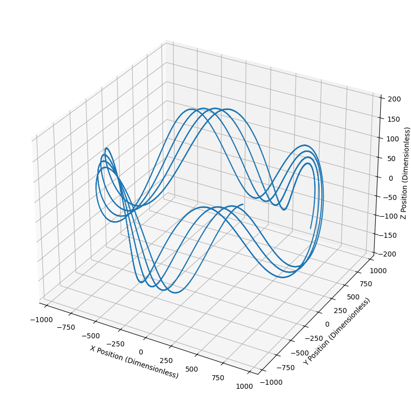
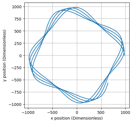
The addition of a poloidal field adds a periodic poloidal motion to the trajectory. The amplitude of the particle’s oscillation in the z-direction does not grow with time, so the drift has been mitigated.
I’ve only provided the analytic form of these drifts to keep this short. If you’re looking for a conceptual understanding, I suggest chapter 4 of “The Future of Fusion Energy” by Parisi and Ball. For an introduction to the Runge-Kutta method, see Chapter 6 of Toby Driscoll’s “Fundamentals of Numerical Computation”.